GEOG 2700 Fall 2018: Statistical Analysis and Hypothesis Testing

This GEOG 2700 Fall 2018 independent assessment solution provides detailed answers to questions related to statistical analysis and hypothesis testing. It covers topics such as calculating probabilities of events (vehicle accidents, lightning-related fires), determining quantiles for normally and t-distributed variables, defining sampling strategies, understanding sample statistics and the central limit theorem, and constructing confidence intervals for proportions and means. Furthermore, it includes step-by-step solutions for hypothesis tests, including one-sample proportion z-tests, one-sample t-tests, and F-tests for variances, with clear explanations of each step and the interpretation of results. Desklib offers this and many more solved assignments to help students excel.

GEOG 2700
Fall 2018 Independent Assessment2
1

PART 1
1.01
You have observed that the probability of a vehicle accident occurring at a particular intersection is 1/10.
If you drive through this intersection 10 times per week, what is the probability that you will be involved in
an accident in any given week?
Let p = probability of accident occurring = 1/10, n = drive through this intersection = 10 times per week, and
X = Number of accidents in a week. Hence, required probability of involving in an accident =
P ( X >0 ) =1−P ( X=0 ) =
1− ( 10 C0 )∗( 1
10 )
0
∗( 9
10 )
10
=1− ( 0 . 9 ) 10=0 . 6513
1.02
You have been hired to determine the probability of a lightning-related fire within a local grassland
preserve that covers 10 km2. You have observed that lightning strikes occur with equal probability
everywhere within your management area, and that the likelihood of a lightning strike in any given 1 k2
area is 1/20. You have also observed that probability of a lightning strike resulting in a fire is 0.25. What is
the? You can assume that any lightning strike will result in a fire.
Let, L = lightning strikes, F = fire will occur in the grassland. Now, P ( L ) = 1
20 =0 .05 and P ( F / L ) =0 . 25 .
Therefore, P ( F∩L ) =0 .05∗0 . 25=0 . 0125 = probability that a lightning-related fire will occur in any 1 km2.
Total grassland preserve = 10 km2. Hence, n = 10. Now, required probability of lightning-related fire will
occur in the grassland preserve = P ( X >0 ) =1−P ( X=0 ) =
1− ( 10 C0 )∗( 0 . 0125 ) 0∗( 0 . 9875 ) 10=1− ( 0 .9875 ) 10=0 .1182
1.03
Given a normally distributed random variable X with a mean of 10 and standard deviation of 2, what value
represents the lower 60% quantile of this variable?
Given that X ~ N ( 10 ,22 ) , Hence according to the problem P ( X < x ) =0 . 6
So,
P ( Z< x−10
2 )=0 . 6=P ( Z< 0. 25335 ) => x =10+2∗0 . 25335=10 . 5067≃10 . 51
Hence, x = 10.51 represents the lower 60% quantile.
2

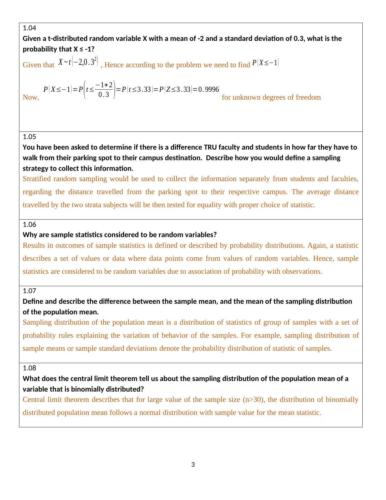
1.04
Given a t-distributed random variable X with a mean of -2 and a standard deviation of 0.3, what is the
probability that X ≤ -1?
Given that X ~ t (−2,0 . 32 ) , Hence according to the problem we need to find P ( X≤−1 )
Now,
P ( X≤−1 ) =P ( t≤−1+ 2
0 . 3 )=P ( t≤3 .33 ) =P ( Z≤3 . 33 ) =0. 9996
for unknown degrees of freedom
1.05
You have been asked to determine if there is a difference TRU faculty and students in how far they have to
walk from their parking spot to their campus destination. Describe how you would define a sampling
strategy to collect this information.
Stratified random sampling would be used to collect the information separately from students and faculties,
regarding the distance travelled from the parking spot to their respective campus. The average distance
travelled by the two strata subjects will be then tested for equality with proper choice of statistic.
1.06
Why are sample statistics considered to be random variables?
Results in outcomes of sample statistics is defined or described by probability distributions. Again, a statistic
describes a set of values or data where data points come from values of random variables. Hence, sample
statistics are considered to be random variables due to association of probability with observations.
1.07
Define and describe the difference between the sample mean, and the mean of the sampling distribution
of the population mean.
Sampling distribution of the population mean is a distribution of statistics of group of samples with a set of
probability rules explaining the variation of behavior of the samples. For example, sampling distribution of
sample means or sample standard deviations denote the probability distribution of statistic of samples.
1.08
What does the central limit theorem tell us about the sampling distribution of the population mean of a
variable that is binomially distributed?
Central limit theorem describes that for large value of the sample size (n>30), the distribution of binomially
distributed population mean follows a normal distribution with sample value for the mean statistic.
3

1.09
State the equations that define the sampling distribution of the population proportion. Make sure to
define each variable that appears in these equations.
Equations defining the requisite distribution will be μ= p
^¿
¿ and
σ ¿ ¿ , where p
^¿
¿ the sample
proportion and “n” is is the sample size. The population proportion is distributed with mean μ and standard
deviation σ .
1.10
You are the manager of a popular restaurant. You have been asked to estimate the proportion of
customers who have food allergies. To do this, you sample 150 customers at random and find that 17 of
them have food allergies. Determine the 95% confidence interval of the proportion of customers at your
restaurant who have food allergies. Write out all relevant equations and state your confidence interval as:
According to the problem, n=150 , p=17
150 =0. 113 . The 95% confidence interval of the proportion of
customers is calculated as CI =p±z0. 025∗
√ p ( 1− p )
n =0 . 113±1 . 96∗ √ 0 .113∗0 . 887
150 =[0 . 063 , 0. 163 ] . Hence,
0 . 063≤π≤0. 163 and it is estimated that proportion of customers with food allergies will be somewhere
between 0.063 and 0.163
1.11
You have been asked to estimate the cost of living of TRU students who live in off-campus apartments. In
a random sample of 300 students, you find that the mean cost of living is$1,200 per month with a standard
deviation of 50. Determine the 90% confidence interval of the cost of living for TRU students. Write out
all relevant equations and state your confidence interval as:
According to the problem, n=150 , x
¿
=1200 , s=50
So the 90% confidence interval was evaluated using the formula
CI =x
−
±t0. 05∗ s
√ n =1200±1 . 64∗50
√ 150 =[1193 . 28 ,1206 . 72] where t-statistics was calculated for 149
degrees of freedom for the probability of 0.90 within the confidence interval. Hence,
1193. 28≤μ≤1206 . 72 estimates the population mean with 90% confidence.
4

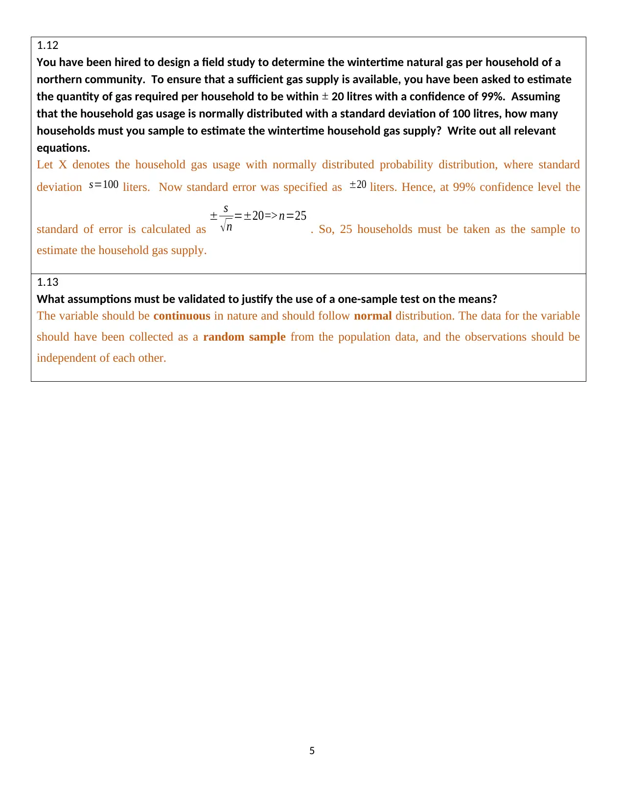
1.12
You have been hired to design a field study to determine the wintertime natural gas per household of a
northern community. To ensure that a sufficient gas supply is available, you have been asked to estimate
the quantity of gas required per household to be within ± 20 litres with a confidence of 99%. Assuming
that the household gas usage is normally distributed with a standard deviation of 100 litres, how many
households must you sample to estimate the wintertime household gas supply? Write out all relevant
equations.
Let X denotes the household gas usage with normally distributed probability distribution, where standard
deviation s=100 liters. Now standard error was specified as ±20 liters. Hence, at 99% confidence level the
standard of error is calculated as
± s
√ n =±20=> n=25
. So, 25 households must be taken as the sample to
estimate the household gas supply.
1.13
What assumptions must be validated to justify the use of a one-sample test on the means?
The variable should be continuous in nature and should follow normal distribution. The data for the variable
should have been collected as a random sample from the population data, and the observations should be
independent of each other.
5

1.14
You have been hired to evaluate the claim that the less than 25% of TRU students hold full-time
employment outside of TRU. To do this, you randomly sample 150 TRU students and find that 30 of them
hold full-time employment outside of TRU.
(1) State what type of statistical hypothesis test would you to test this assertion.
(2) Use the 6-step procedure demonstrated in class to test the assertion that less than 25% of TRU
students hold full-time employment outside of TRU at a significance level of 5%. Write out each of
the 6-steps, including all relevant equations, and clearly state the outcome of the test.
Size of sample = n=150 and the sample proportion is p
^¿= 3
15 = 1
5
¿ =0.2
(1) The claim can be tested by a left tail alternate hypothesis at 5% level of significance by z-test for one
sample proportion.
(2) Step 1: The null hypothesis H0: ( p=0 . 25 )
Step 2: Alternate hypothesis HA: ( p<0 .25 )
Step 3: Level of significance α=5 %=0 . 05
Step 4: Choice of test: One sample z-test.
z−stat= p
^¿− p
√ p(1− p )
n
= 0 . 2−0 . 25
√ 0 . 25∗0 .75
150
=−1 . 414 ¿
Step 5: The p-value is calculated as P ( z <−1 . 414 ) =0 . 0786
Step 6: The p-value was greater than α=0 . 05 and the null hypothesis failed to get rejected. Hence, the
proportion was not significantly less than 0.25.
6

1.15
You have been hired to determine whether the average snow depth at a ski resort exceeds 2 meters. To
do this you measure the snow depth in cm at 30 random locations throughout the resort. These data are
approximately normally distributed, with a mean of 210 cm and a standard deviation of 30 cm.
(1) What type of statistical hypothesis test would you use to test this assertion?
(2) Use the 6-step procedure demonstrated in class to test the assertion that the snow depth is greater
than 2 m at a significance level of 5%. Write out each of the 6-steps, including all relevant
equations, and clearly state the outcome of the test.
Size of sample = 30 and the sample mean is x
¿
=210 and s=30
(1) The claim can be tested by a right tail alternate hypothesis at 5% level of significance by one sample t-
test.
(2) Step 1: The null hypothesis H0: ( μ=200 )
Step 2: Alternate hypothesis HA: ( μ>200 )
Step 3: Level of significance α=5 %=0 . 05
Step 4: Choice of test: One sample t-test.
t−stat = x
¿
−μ
s
√ n
=210−200
√ 30
30
=1 . 826
Step 5: The p-value is calculated as P ( t >1 .826 ) =0 . 0391
Step 6: The p-value was less than α=0 . 05 and the null hypothesis is rejected. Hence, it is concluded that there
is statistical significant evidence that snow depth at a ski resort exceeds 2 meters.
7

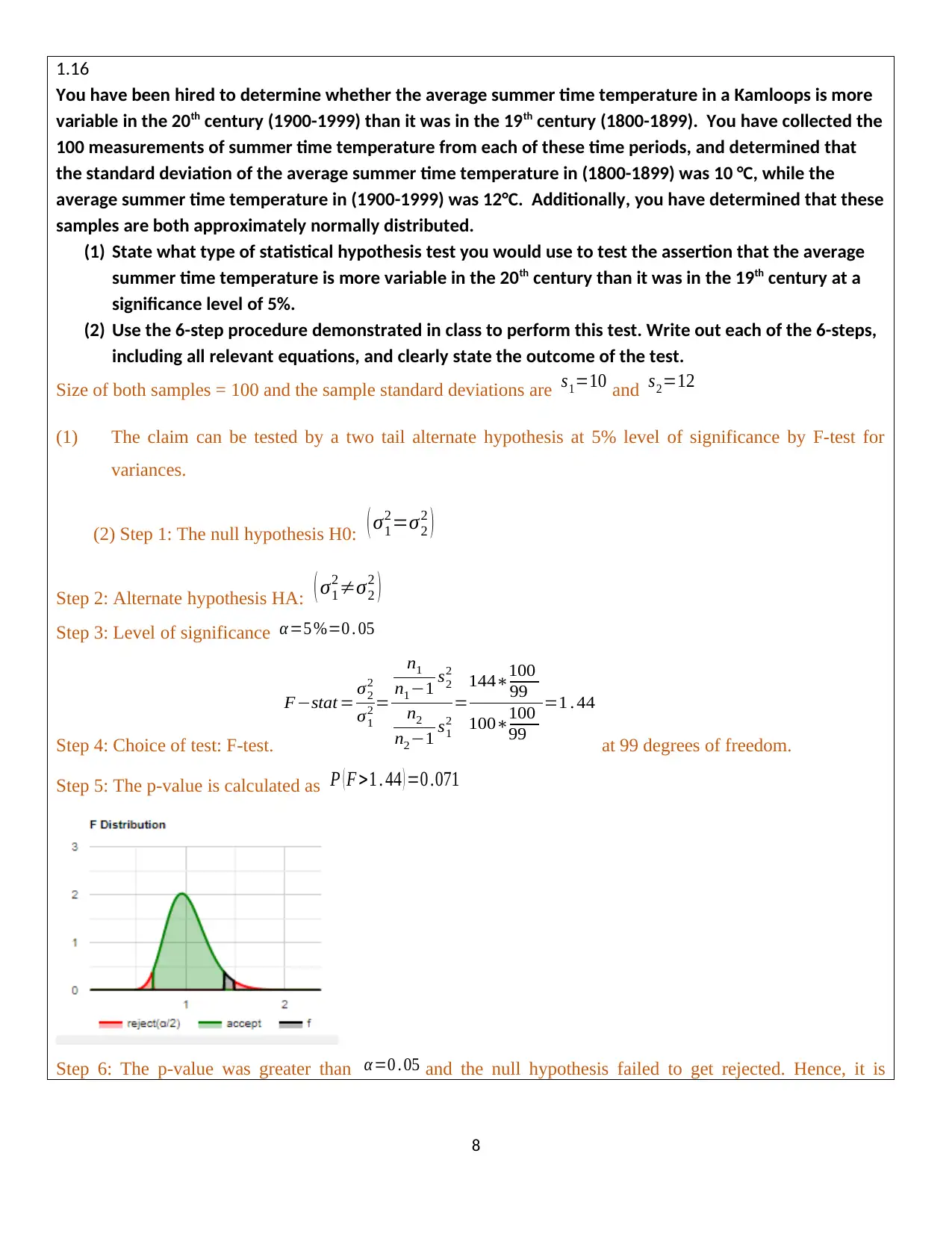
1.16
You have been hired to determine whether the average summer time temperature in a Kamloops is more
variable in the 20th century (1900-1999) than it was in the 19th century (1800-1899). You have collected the
100 measurements of summer time temperature from each of these time periods, and determined that
the standard deviation of the average summer time temperature in (1800-1899) was 10 °C, while the
average summer time temperature in (1900-1999) was 12°C. Additionally, you have determined that these
samples are both approximately normally distributed.
(1) State what type of statistical hypothesis test you would use to test the assertion that the average
summer time temperature is more variable in the 20th century than it was in the 19th century at a
significance level of 5%.
(2) Use the 6-step procedure demonstrated in class to perform this test. Write out each of the 6-steps,
including all relevant equations, and clearly state the outcome of the test.
Size of both samples = 100 and the sample standard deviations are s1=10 and s2=12
(1) The claim can be tested by a two tail alternate hypothesis at 5% level of significance by F-test for
variances.
(2) Step 1: The null hypothesis H0: ( σ1
2=σ2
2 )
Step 2: Alternate hypothesis HA: ( σ1
2≠σ2
2 )
Step 3: Level of significance α=5 %=0 . 05
Step 4: Choice of test: F-test.
F−stat = σ2
2
σ1
2 =
n1
n1−1 s2
2
n2
n2−1 s1
2
=
144∗100
99
100∗100
99
=1 . 44
at 99 degrees of freedom.
Step 5: The p-value is calculated as P ( F >1 . 44 ) =0 .071
Step 6: The p-value was greater than α=0 . 05 and the null hypothesis failed to get rejected. Hence, it is
8

concluded that there is not enough statistical significant evidence for difference in variation in summer
temperature between the two time periods.
9

1.17
A restaurant has hired you to determine whether a recent change in their menu has increased their
average daily revenue by at least $500. They have provided you with two samples of their daily revenue,
both of which are approximately normally distributed.One sample consists of 65 daily revenue values,
randomly sampled from the period before the change. This sample has a mean of $5,100 with a standard
deviation of $300. The second sample consists of 36 daily revenue values, sampled at random from the
period following the change. This sample has a mean of $5,750, with a standard deviation of $600.
(1) State what type of statistical hypothesis test you would use to test the assertion that the daily
revenue has increased by at least $500 at a significance level of 5%.
(2) Use the 6-step procedure demonstrated in class to test to perform this test. Write out each of the
6-steps, including all relevant equations, and clearly state the outcome of the test.
Size of samples are n1=65 , n2=36
Sample means are x
¿
1=5100 , x
¿
2=5750 standard deviations are s1=300 and s2=600
(1) The claim can be tested by a right tail alternate hypothesis at 5% level of significance by t-test for
difference between means.
(2) Step 1: The null hypothesis H0: ( μ2−μ1=μd=500 )
Step 2: Alternate hypothesis HA: ( μ2−μ1>500 )
Step 3: Level of significance α=5 %=0 . 05
Step 4: Choice of test: t-test for difference.
t−stat = x2−x1−μd
SE =5750−5100−500
106 .70 =0 .9372 where pooled standard deviation is
SE= √ s1
2
n1
+ s2
2
n2
= √ 3002
65 + 6002
36 =106 .70
Step 5: The p-value is calculated as P ( t >0 . 9372 ) =0 . 1768
Step 6: The p-value was greater than α =0 . 05 and the null hypothesis failed to get rejected. Hence, it is
concluded that there is not enough statistical significant evidence to claim that sales have increased by
at least $ 500.
10

1.18
The city centreneighbourhood is changing as people increasingly choose to live downtown to be closer to
their places of employment. A study from 1979 reveals that from a random sample of 500 residential
properties, 470 of them were multi-family residences. From the 2010 census data, you determine that
from a random sample of 760 residential properties, 605 of them were multi-family residences. You would
like to evaluate the assertion that the proportion of multi-family residences has decreased by at least 10%
between 1979 and 2010.
(1) State what type of statistical hypothesis you would use to test the assertion that the proportion of
multi-family residences has decreased by at least 10% between 1979 and 2010 at a significance level
of 5%.
(2) Use the 6-step procedure demonstrated in class to test to perform this test. Write out each of the 6-
steps, including all relevant equations, and clearly state the outcome of the test.
Size of sample is n1=500 and the sample proportion is p
^¿1=47
50 =0. 94
¿ and n 2=760 and the sample proportion
is p
^¿2=605
760 =0 .796
¿
(1) The claim can be tested by a right tail alternate hypothesis at 5% level of significance by z-test for
difference of two sample proportions.
(2) Step 1: The null hypothesis H0: ( p1− p2=pd=0 . 1 )
Step 2: Alternate hypothesis HA: ( p1− p2=pd >0 .1 )
Step 3: Level of significance α=5 %=0 . 05
Step 4: Choice of test: z-test. z−stat= p
^¿1− p
^¿
2−p
d
SE
=0 . 94−0 . 796−0. 1
SE =2. 718 ¿ ¿ Where pooled standard
deviation is
SE= √ p1 ( 1− p1 )
n1
+ p2 ( 1−p2 )
n1
= √ 0 .94∗0. 06
500 + 0 .796∗0 . 204
760 =0 . 0162
Step 5: The p-value is calculated as P ( z >2 .718 ) < 0 .001
Step 6: The p-value was way less than α =0 . 05 and the null hypothesis is rejected. Hence, proportion of multi-
family residences has decreased significantly by at least 10%.
11

1.19
In order to perform parametric statistical tests, you must first demonstrate that the variable(s) that will be
tested are approximately normally distributed. Of the tests we have learned in class, which type of
statistical test could you use to evaluate whether or not the assumption that the variable(s) are
approximately normally distributed is valid?
Type of statistical tests that could be used to evaluate the normality assumption of the variable are: Shapiro
Wilk test and Kolmogorov–Smirnov test.
1.20
One of the assumptions required to apply a t-test on the sample mean is that the sample data are
independent. Of the tests we have learned in class, which type of test could you use to evaluate this
assumption?
Correlation test or Scatter plot can be used to test that the sample data are independent.
1.21
Why are non-parametric tests preferable for evaluating hypotheses regarding Likert scale variables?
Likert scale variable responses are ordinal in nature where the numbers associated with the options are not
meaningful. Hence, for sample size less than 30 will ne not normal in nature. But, sometimes for interval scale
Likert data with observations greater than 30, parametric tests can be used.
1.22
You have been hired by a client to evaluate the claim that Kamloops’ air quality does not meet Federal air
quality standards. To do this you measure the amount of air pollution present every day for 2 years.
Unfortunately, these data are highly non-normal and cannot be transformed into a nearly normal variable.
Of the tests we have learned in class, which type of statistical test could you perform using these data to
support an assertion that the air quality does not meet the air quality standards?
For non-normal variable, Non-parametric tests such as Wilcoxon Signed Rank test, Mann–Whitney U test, and
Kruskal-Wallis test are used.
12