BUS708 Statistical Analysis and Modeling of NSW Transport Data

This report presents a statistical analysis of the New South Wales (NSW) transport system, utilizing both provided secondary data and newly collected primary data. The analysis includes frequency distributions, one-sample Z-tests, two-sample t-tests, and Chi-square tests to address specific research questions related to transportation mode preferences, railway line construction, and gender-based transportation choices. Key findings indicate that buses are the most preferred mode of transport, Parramatta is the busiest railway station, and there is no significant difference in transportation mode preference between genders. The report concludes with recommendations for NSW government, including improvements to ferry and light-rail systems and the construction of a new railway line between Parramatta and Central. The analyses were conducted using MS Excel-2016 software. The primary data was collected via survey while the secondary data was provided by the organization.

Running Head: STATISTICS
Statistics
Name of the student:
Name of the university:
Course ID:

1STATISTICS
Table of Contents
1. First Section: Introduction and Background:.....................................................................................2
2. Second Section: Analysis of Single variable in First Data set:.............................................................2
3. Third Section: Analysis of Double variable in First Data set:..............................................................5
4. Fourth Section: Collection and Analysis of Second Data set:.............................................................7
5. Fifth Section: Discussion and Conclusion:..........................................................................................8
References:............................................................................................................................................9
Table of Figures
Figure 1: Frequency distribution of transportation mode.....................................................................3
Figure 2: Frequency distribution of trains as per Locations...................................................................6
Figure 3: Grouped bar plot of frequency of passengers of various ways as per gender........................8
Table of tables
Table 1: Transportation used by New South Wales...............................................................................3
Table 2: One-sample Z-test....................................................................................................................4
Table 3: Frequency table of trains as per Locations...............................................................................5
Table 4: Table of two-sample t-test assuming unequal variances.........................................................6
Table 5: Gender wise distribution of transportation passengers according to the types of vehicles....7
Table 6: Chi-square test of association..................................................................................................7

2STATISTICS
1. First Section: Introduction and Background:
1. a)
The transportation is the New South Wales is the leading agency of the New South Wales
transportation cluster. The role is transportation is to establish a more efficient, safer and integrated
transportation system (Amiril et al. 2014). The transportation system majorly keeps people moving
and links the communities of the centers, suburbs, regions and cities. The well-known types of
transportation system of New South Wales are ‘rail’, ‘bus’, ‘light rail’ and ‘ferry’. Public and people
who are equally associated to the transportation system, are equally responsible for planning, policy,
regulation, strategy, allocation of funding and non-service delivery functions.
The transportation system focuses to enhance the ‘customer experience’ and links the
‘public and private operators’ for delivering customer-oriented transport services on their behalf
(Ghaderi et al. 2015). The procurement of transport infrastructure and delivery through ‘project
delivery industry’ are maintained by co-ordination of all people in the New South Wales.
1. b)
The first data set that is provided by my organization is secondary data. The data is collected
by other person and now I am using the data in this statistical documentation. Therefore, the data
set is secondary to me. Although, the data set could be biased and erroneous, I am performing the
analysis with that secondary data with true belief.
The variables that are involved in the data set is qualitative as well as quantitative. The first
variable ‘Mode’ is the indicator of mode of transportation that is nominal (categorical) variable. It
has four levels that are ‘Bus’, ‘Train’, ‘Ferry’ and ‘Light Rail’ (Clark 2013). The second variable ‘Date’
refers the date given in Date/month/year notation. It is another nominal (categorical) data. The
dates are from 8th August, 2016 to 14th August, 2014. ‘Tap’ variable has two levels that are ‘On’ and
‘Off’. It is another nominal (categorical) data. ‘loc’ variable denotes the location of stops in New
South Wales (for bus postcodes and other names of the stations). ‘count’ variable denotes the total
number of tap on and tap off on the certain location and certain date. It is the quantitative variable.
1. c)
I have collected the data set by survey method. The target population was the common
population of New South Wales who travel by transportation services. The data of only gender and
transportation data is collected in this regard. The data set is primary data as I myself have collected
the data set. The variables of the new collected data set are qualitative in nature. However, the
number of samples of the data set is not adequately large. Also, the primary data set has only two
variables; hence, it is in-sufficient and inadequate.
2. Second Section: Analysis of Single variable in First Data set:
2. a)

3STATISTICS
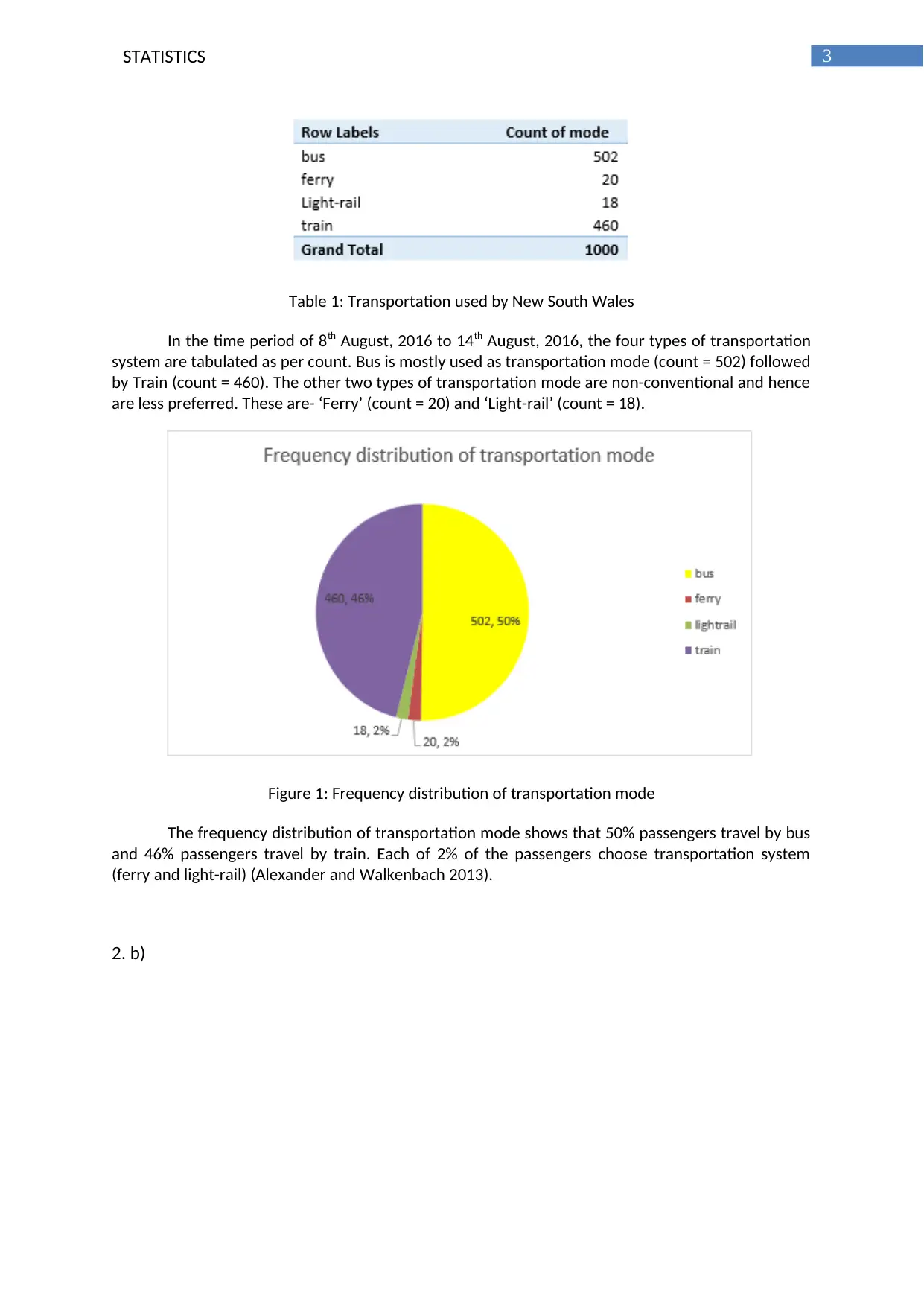
Table 1: Transportation used by New South Wales
In the time period of 8th August, 2016 to 14th August, 2016, the four types of transportation
system are tabulated as per count. Bus is mostly used as transportation mode (count = 502) followed
by Train (count = 460). The other two types of transportation mode are non-conventional and hence
are less preferred. These are- ‘Ferry’ (count = 20) and ‘Light-rail’ (count = 18).
Figure 1: Frequency distribution of transportation mode
The frequency distribution of transportation mode shows that 50% passengers travel by bus
and 46% passengers travel by train. Each of 2% of the passengers choose transportation system
(ferry and light-rail) (Alexander and Walkenbach 2013).
2. b)

4STATISTICS
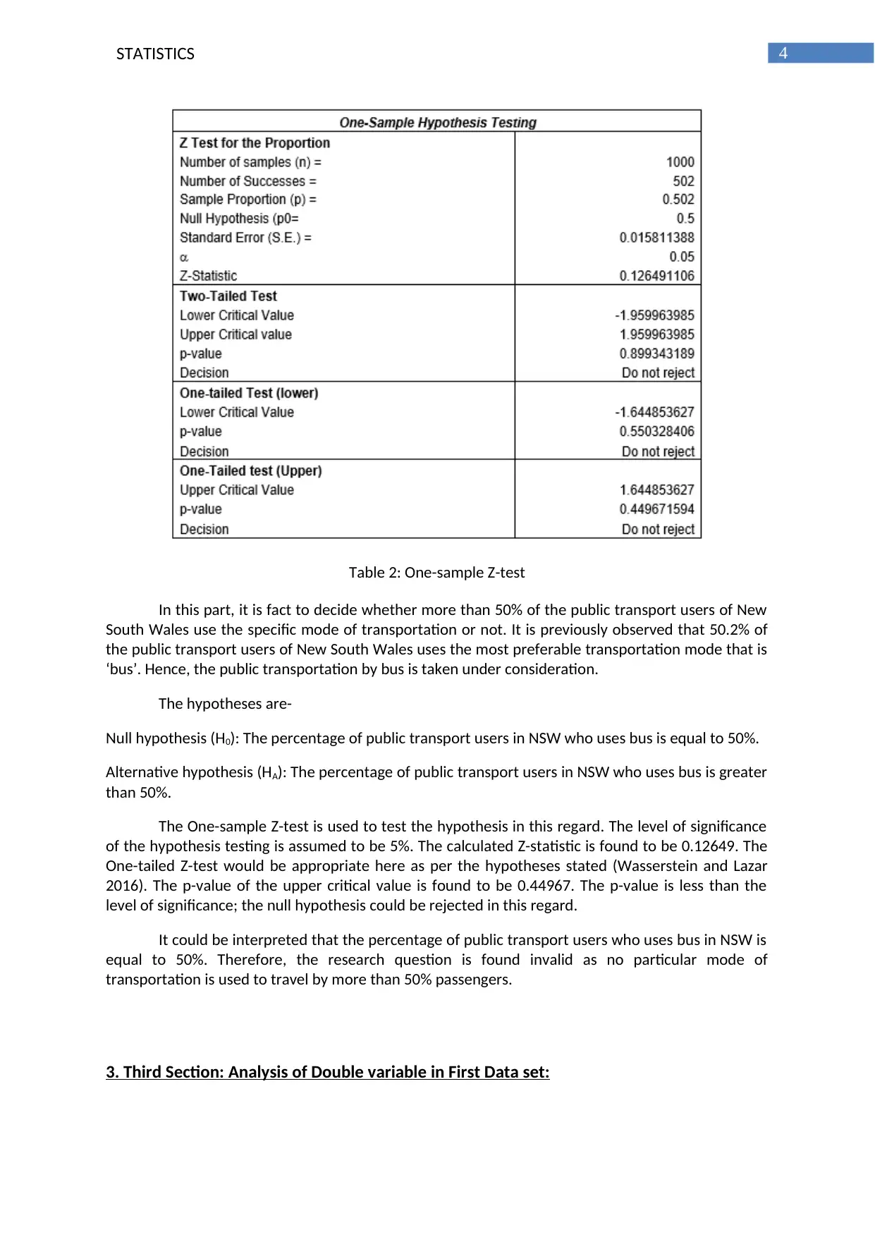
Table 2: One-sample Z-test
In this part, it is fact to decide whether more than 50% of the public transport users of New
South Wales use the specific mode of transportation or not. It is previously observed that 50.2% of
the public transport users of New South Wales uses the most preferable transportation mode that is
‘bus’. Hence, the public transportation by bus is taken under consideration.
The hypotheses are-
Null hypothesis (H0): The percentage of public transport users in NSW who uses bus is equal to 50%.
Alternative hypothesis (HA): The percentage of public transport users in NSW who uses bus is greater
than 50%.
The One-sample Z-test is used to test the hypothesis in this regard. The level of significance
of the hypothesis testing is assumed to be 5%. The calculated Z-statistic is found to be 0.12649. The
One-tailed Z-test would be appropriate here as per the hypotheses stated (Wasserstein and Lazar
2016). The p-value of the upper critical value is found to be 0.44967. The p-value is less than the
level of significance; the null hypothesis could be rejected in this regard.
It could be interpreted that the percentage of public transport users who uses bus in NSW is
equal to 50%. Therefore, the research question is found invalid as no particular mode of
transportation is used to travel by more than 50% passengers.
3. Third Section: Analysis of Double variable in First Data set:

5STATISTICS
3. a)
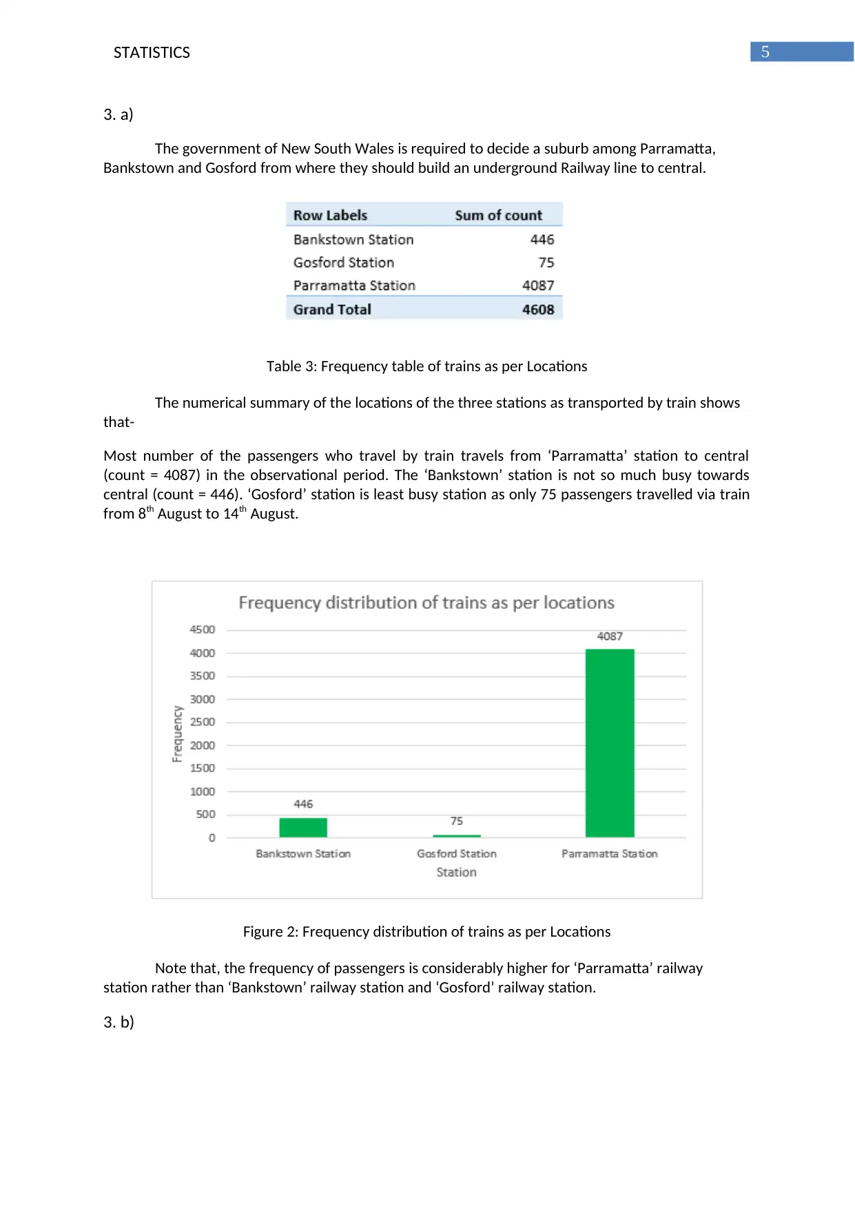
The government of New South Wales is required to decide a suburb among Parramatta,
Bankstown and Gosford from where they should build an underground Railway line to central.
Table 3: Frequency table of trains as per Locations
The numerical summary of the locations of the three stations as transported by train shows
that-
Most number of the passengers who travel by train travels from ‘Parramatta’ station to central
(count = 4087) in the observational period. The ‘Bankstown’ station is not so much busy towards
central (count = 446). ‘Gosford’ station is least busy station as only 75 passengers travelled via train
from 8th August to 14th August.
Figure 2: Frequency distribution of trains as per Locations
Note that, the frequency of passengers is considerably higher for ‘Parramatta’ railway
station rather than ‘Bankstown’ railway station and ‘Gosford’ railway station.
3. b)

6STATISTICS
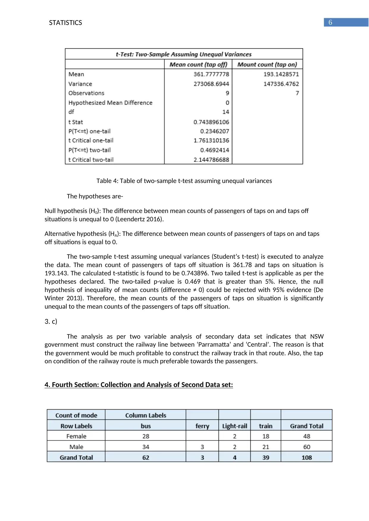
Table 4: Table of two-sample t-test assuming unequal variances
The hypotheses are-
Null hypothesis (H0): The difference between mean counts of passengers of taps on and taps off
situations is unequal to 0 (Leendertz 2016).
Alternative hypothesis (HA): The difference between mean counts of passengers of taps on and taps
off situations is equal to 0.
The two-sample t-test assuming unequal variances (Student’s t-test) is executed to analyze
the data. The mean count of passengers of taps off situation is 361.78 and taps on situation is
193.143. The calculated t-statistic is found to be 0.743896. Two tailed t-test is applicable as per the
hypotheses declared. The two-tailed p-value is 0.469 that is greater than 5%. Hence, the null
hypothesis of inequality of mean counts (difference ≠ 0) could be rejected with 95% evidence (De
Winter 2013). Therefore, the mean counts of the passengers of taps on situation is significantly
unequal to the mean counts of the passengers of taps off situation.
3. c)
The analysis as per two variable analysis of secondary data set indicates that NSW
government must construct the railway line between ‘Parramatta’ and ‘Central’. The reason is that
the government would be much profitable to construct the railway track in that route. Also, the tap
on condition of the railway route is much preferable towards the passengers.
4. Fourth Section: Collection and Analysis of Second Data set:

7STATISTICS
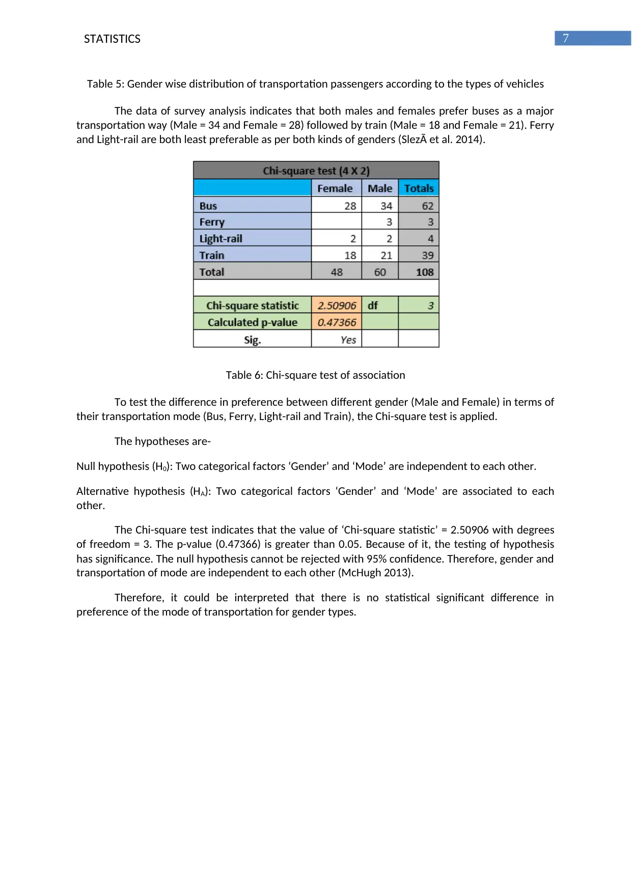
Table 5: Gender wise distribution of transportation passengers according to the types of vehicles
The data of survey analysis indicates that both males and females prefer buses as a major
transportation way (Male = 34 and Female = 28) followed by train (Male = 18 and Female = 21). Ferry
and Light-rail are both least preferable as per both kinds of genders (Slezà et al. 2014).
Table 6: Chi-square test of association
To test the difference in preference between different gender (Male and Female) in terms of
their transportation mode (Bus, Ferry, Light-rail and Train), the Chi-square test is applied.
The hypotheses are-
Null hypothesis (H0): Two categorical factors ‘Gender’ and ‘Mode’ are independent to each other.
Alternative hypothesis (HA): Two categorical factors ‘Gender’ and ‘Mode’ are associated to each
other.
The Chi-square test indicates that the value of ‘Chi-square statistic’ = 2.50906 with degrees
of freedom = 3. The p-value (0.47366) is greater than 0.05. Because of it, the testing of hypothesis
has significance. The null hypothesis cannot be rejected with 95% confidence. Therefore, gender and
transportation of mode are independent to each other (McHugh 2013).
Therefore, it could be interpreted that there is no statistical significant difference in
preference of the mode of transportation for gender types.

8STATISTICS
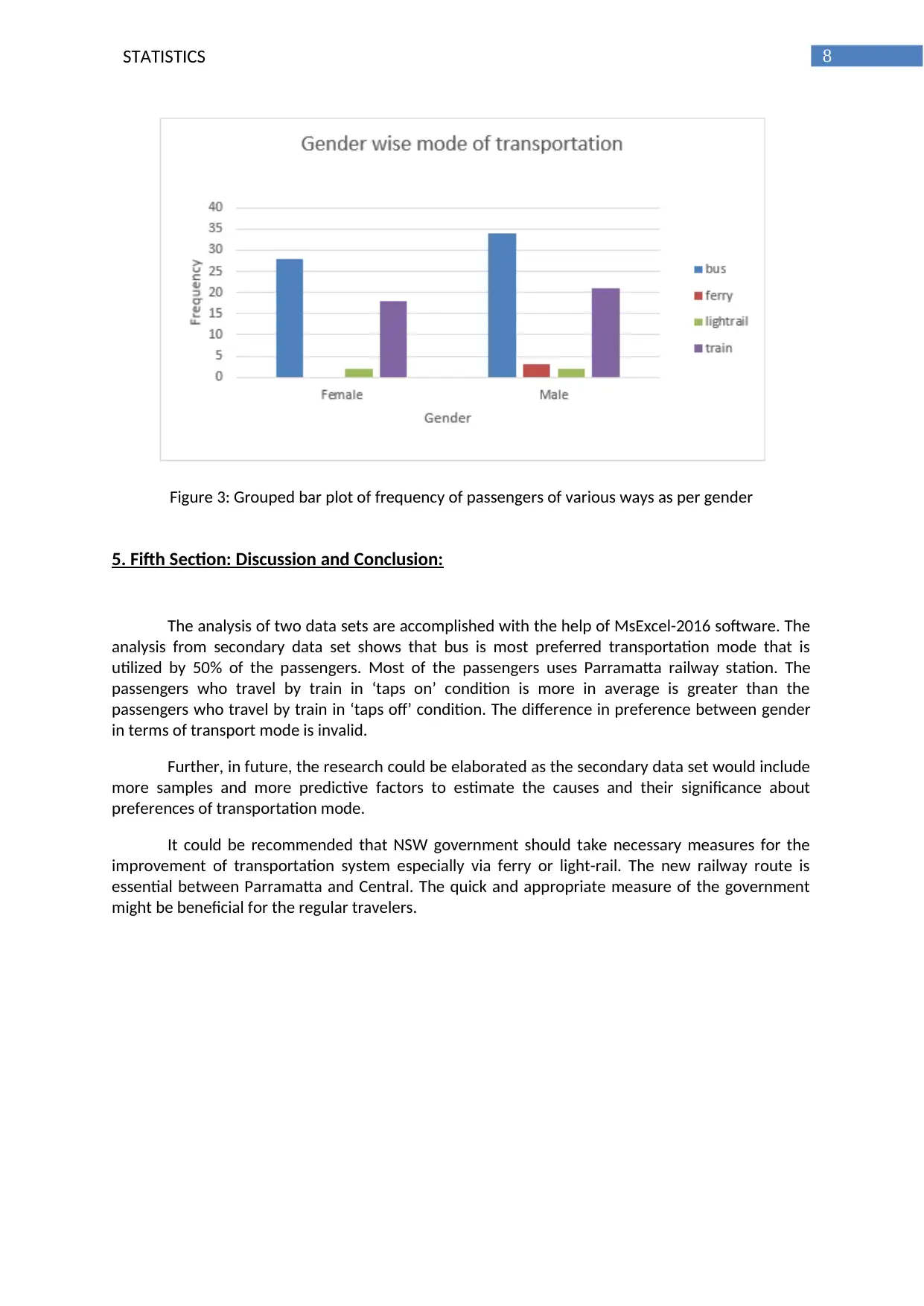
Figure 3: Grouped bar plot of frequency of passengers of various ways as per gender
5. Fifth Section: Discussion and Conclusion:
The analysis of two data sets are accomplished with the help of MsExcel-2016 software. The
analysis from secondary data set shows that bus is most preferred transportation mode that is
utilized by 50% of the passengers. Most of the passengers uses Parramatta railway station. The
passengers who travel by train in ‘taps on’ condition is more in average is greater than the
passengers who travel by train in ‘taps off’ condition. The difference in preference between gender
in terms of transport mode is invalid.
Further, in future, the research could be elaborated as the secondary data set would include
more samples and more predictive factors to estimate the causes and their significance about
preferences of transportation mode.
It could be recommended that NSW government should take necessary measures for the
improvement of transportation system especially via ferry or light-rail. The new railway route is
essential between Parramatta and Central. The quick and appropriate measure of the government
might be beneficial for the regular travelers.

9STATISTICS
References:
Alexander, M. and Walkenbach, J., 2013. Excel dashboards and reports (Vol. 17). John Wiley & Sons.
Amiril, A., Nawawi, A.H., Takim, R. and Latif, S.N.F.A., 2014. Transportation infrastructure project
sustainability factors and performance. Procedia-Social and Behavioral Sciences, 153, pp.90-98.
Clark, G., 2013. 5 Secondary data. Methods in Human Geography, p.57.
De Winter, J.C., 2013. Using the Student's t-test with extremely small sample sizes. Practical
Assessment, Research & Evaluation, 18(10).
Ghaderi, H., Namazi-Rad, M.R., Cahoon, S. and Fei, J., 2015. Improving the quality of rail freight
services by managing the time-based attributes: the case of non-bulk rail network in Australia. World
Review of Intermodal Transportation Research, 5(3), pp.203-220.
Leendertz, S.A.J., 2016. Testing new hypotheses regarding ebolavirus reservoirs.
McHugh, M.L., 2013. The chi-square test of independence. Biochemia medica: Biochemia
medica, 23(2), pp.143-149.
Slezà P, Bokes P, Pavol NÃ, WaczulÃkovà I, 2014. Microsoft Excel add-in for the statistical analysis of
contingency tables. International Journal for Innovation Education and Research. 2(5):90-100.
Wasserstein, R.L. and Lazar, N.A., 2016. The ASA’s statement on p-values: context, process, and
purpose. The American Statistician, 70(2), pp.129-133.