Application of Statistical Methods in Business Decision-Making
VerifiedAdded on 2020/06/04
|18
|3321
|200
AI Summary
The report investigates how organizations utilize statistical techniques, particularly focusing on the Economic Order Quantity (EOQ), to make informed decisions about inventory management. By examining case studies and theoretical models, students assess the impact of EOQ on minimizing costs and optimizing resource allocation. The analysis includes evaluating different types of charts and data interpretations used in business statistics, providing insights into effective decision-making processes.

Statistic for management
Paraphrase This Document
Need a fresh take? Get an instant paraphrase of this document with our AI Paraphraser
Table of Contents
INTRODUCTION...........................................................................................................................1
TASK 1............................................................................................................................................1
Evaluation of economic and business data:...............................................................................1
a). Change in gross annual earnings in the public and the private sector since 2009.................1
b). Gap between male and female annual earnings:....................................................................3
TASK 2............................................................................................................................................5
A). Analyse raw firm by implementing statistical tools:............................................................5
B. Comparative analysis:............................................................................................................8
A). Scatter diagram:....................................................................................................................8
b). Equation on scatter line:......................................................................................................10
c) Calculation of total turnover.................................................................................................10
d).Correlation Coefficient:........................................................................................................10
e). Statistical validity:................................................................................................................11
TASK 3..........................................................................................................................................11
A). Number of delivery in a current year;.................................................................................11
B. Number of bottles delivery delivered with each delivery:...................................................11
C. Calculation of EOQ:.............................................................................................................12
D. Comparison between current operating model and economic order quantity:....................12
TASK 4..........................................................................................................................................14
a) Scatter diagram:....................................................................................................................14
b). Line chart:............................................................................................................................14
C). Ogive graph:........................................................................................................................15
CONCLUSION:.............................................................................................................................15
REFERENCES..............................................................................................................................16

⊘ This is a preview!⊘
Do you want full access?
Subscribe today to unlock all pages.
Trusted by 1+ million students worldwide
INTRODUCTION
Statistics is the major tool which is used to analyse the firm financial performance. There
are so many tools which are used for assessing the performance of the company. By using
statistics, company can depicts complicated data into simplest form so that the general public can
analyse the data and also able to draw a valid conclusion. Such report aims at assessing firm
outcomes for assessing their development (Beardwell and Thompson, 2014). Such report aims at
assessing firm outcomes via applying numerous statistical methods in order to frame efficient
decision making. With the help of statistics, company is able to analyse various charts, graphs
and tables, essential findings would be figure out adequately.
TASK 1
Evaluation of economic and business data:
There are basically two kinds of data which are used by the firm for collection, analysing and
assessing for the most specific purpose. These are the data collection methods that can be sued
by the firm in order to formulate various business strategies which would helpful for gaining
competitive advantages. These are Primary data and secondary data.
a). Change in gross annual earnings in the public and the private sector since 2009
According to Office of National Statistics report, the gross annual earnings in the public and
private sector are fluctuating since 2009.
Gross annual earnings for male:
Particulars
Public
sector
Year on
Year
absolute
change
Year-on-
Year
growth
Private
sector
Year on
Year
absolute
change
Year-on-Year
growth
2009 30638 27362
2010 31264 626 2.04% 27000 -362 -1.32%
2011 31380 116 0.37% 27233 233 0.86%
2012 31816 436 1.39% 27705 472 1.73%
2013 32541 725 2.28% 28201 496 1.79%
2014 32878 337 1.04% 28442 241 0.85%
2015 33685 807 2.45% 28881 439 1.54%
2016 34011 326 0.97% 29679 798 2.76%
1
Paraphrase This Document
Need a fresh take? Get an instant paraphrase of this document with our AI Paraphraser
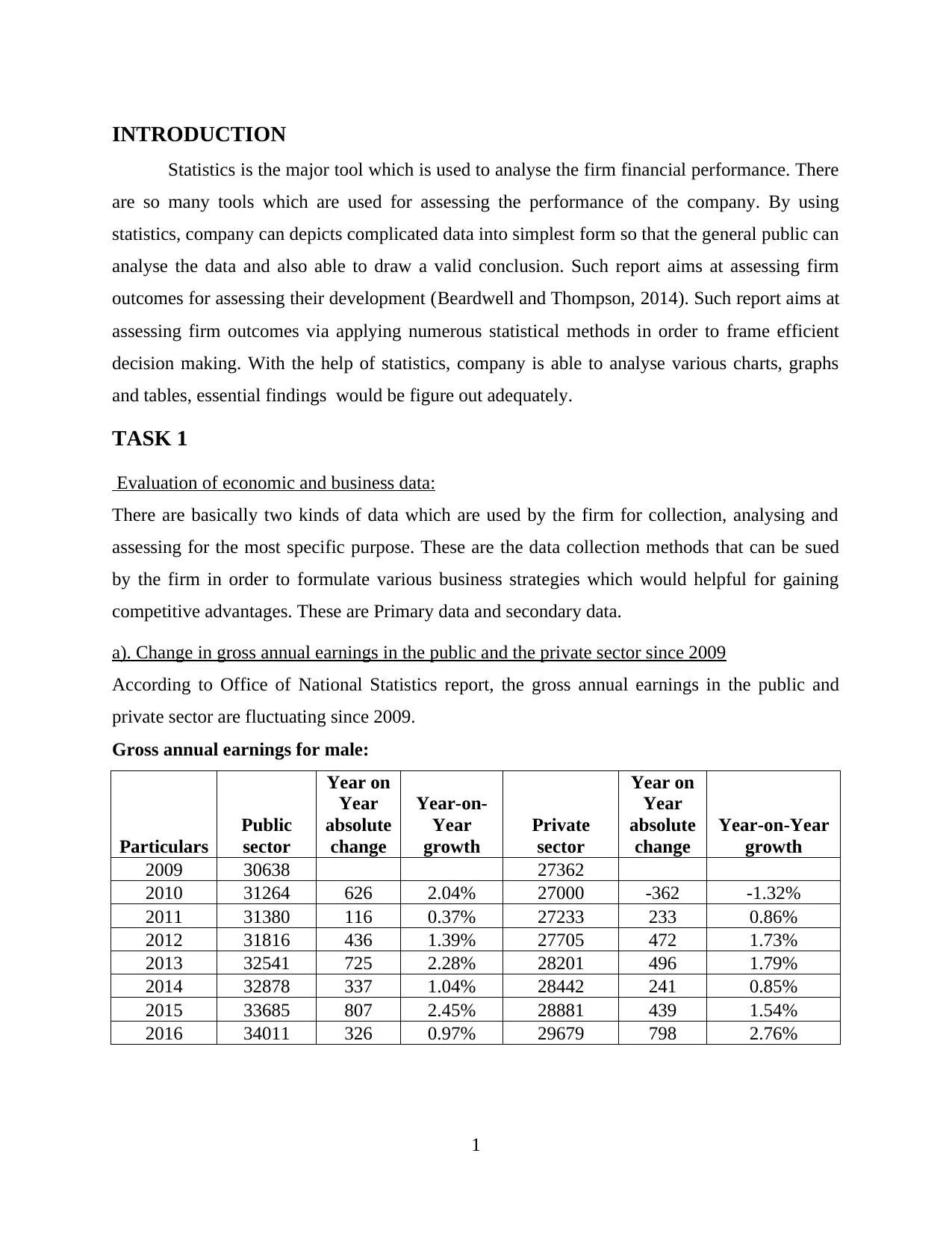
From the above table, this has been observed that the males are continousely increasing but they
are at fluctuating rate, In 2010, this reflects a YOY growth of 2.04% henceforth, reflects lower
enhancement by 0.37%. but this scenario, changed in 2011 and increment in change expend to
1.39%. in 2012, earnings have increasing at sound percentage to 2.28%, which again at less
percentage improvement to 1.04%. Over the period, this has been seen that the earning reflects
the highest growth in 2015 by 2.45%. Although, looking to the private sector, in 2010, gross
annual earnings has been decreased per male from £27,362 to £27,000 by £362 (1.32%)
henceforth, these are used to manage cost, afterwords, 2013 end, it reflects continuously
increasing trends by 0.86%, 1.73% and 1.79% respectively (Embrechts and Hofert, 2014). In the
nest two years, this rose by YOY growth of 0.85% and 1.54%. in 2016, this reflects the highest
increment by 2.76% at earning of £29,679.
Change in the gross annual earnings of Female:
Particulars
Public
sector
Year on
Year
absolute
change
Year-on-
Year
growth
Private
sector
Year on
Year
absolute
change
Year-
on-
Year
growth
2009 25224 19551
2010 26113 889 3.52% 19532 -19 -0.10%
2011 26470 357 1.37% 19565 33 0.17%
2012 26636 166 0.63% 20313 748 3.82%
2013 27338 702 2.64% 20698 385 1.90%
2014 27705 367 1.34% 21017 319 1.54%
2015 27900 195 0.70% 21403 386 1.84%
2016 28053 153 0.55% 22251 848 3.96%
2
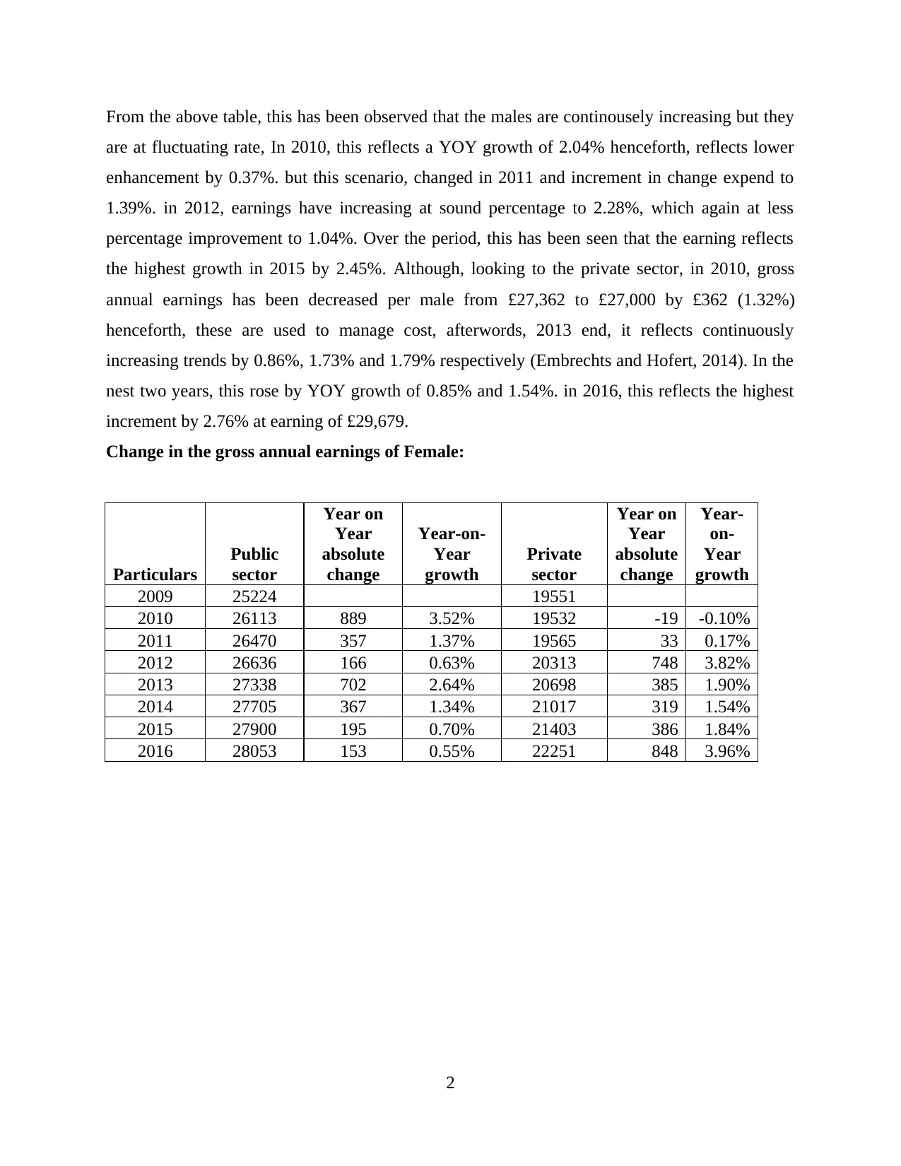
As per the change in the gross annual earnings of female, it has observed that in public sector,
there are various opportunities which are easy to locate from whole female employees. In 2010,
females in the public industry reflects a vast emergence of 3.52% while, in private sector, this
came down to 0.10%. there after, public sector reflects an increasing trends but slow rate by
1.37% and 0.63%, although, private sector reflects an lucrative development by 3.82% in 2012.
From 2014, female employees' in the public sector were getting great salary, whereas YOY
growth is lower in 2014,2015 and 2016 which were 1.34%, 0.70% and 3.96% respectively (Guan
and Zhao, 2012).
b). Gap between male and female annual earnings:
Public sector Male Female Gap
2009 30638 25224 5414
2010 31264 26113 5151
2011 31380 26470 4910
2012 31816 26636 5180
2013 32541 27338 5203
2014 32878 27705 5173
2015 33685 27900 5785
2016 34011 28053 5958
3
⊘ This is a preview!⊘
Do you want full access?
Subscribe today to unlock all pages.
Trusted by 1+ million students worldwide
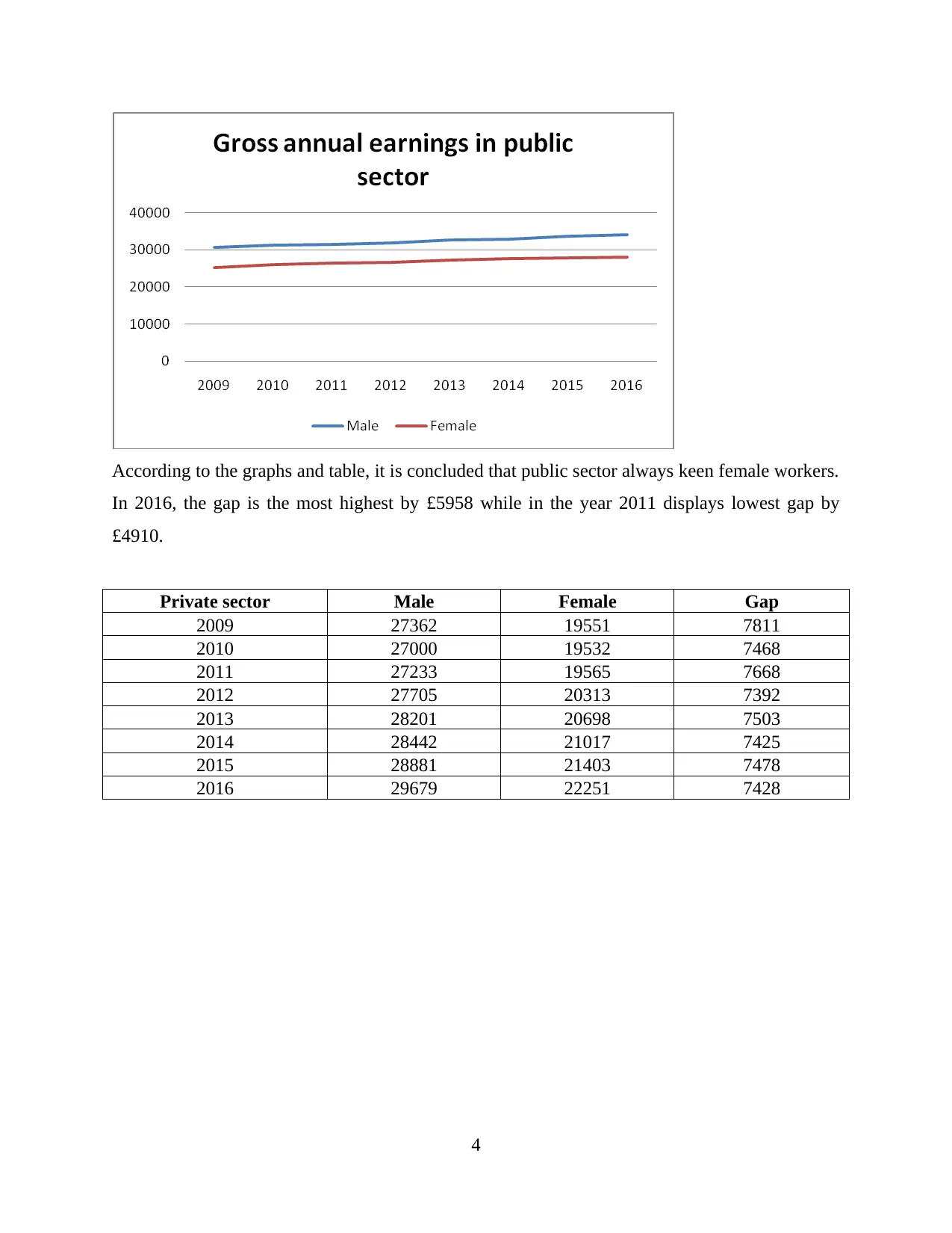
According to the graphs and table, it is concluded that public sector always keen female workers.
In 2016, the gap is the most highest by £5958 while in the year 2011 displays lowest gap by
£4910.
Private sector Male Female Gap
2009 27362 19551 7811
2010 27000 19532 7468
2011 27233 19565 7668
2012 27705 20313 7392
2013 28201 20698 7503
2014 28442 21017 7425
2015 28881 21403 7478
2016 29679 22251 7428
4
Paraphrase This Document
Need a fresh take? Get an instant paraphrase of this document with our AI Paraphraser
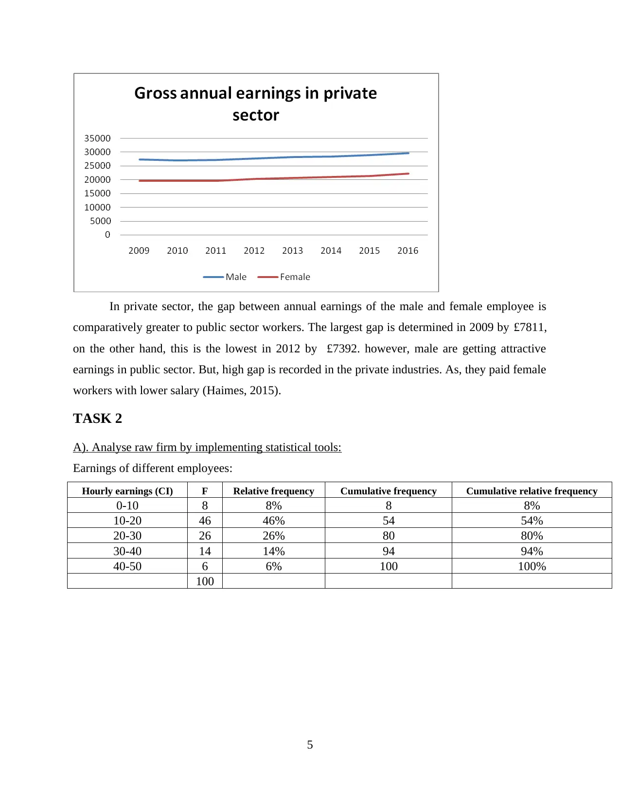
In private sector, the gap between annual earnings of the male and female employee is
comparatively greater to public sector workers. The largest gap is determined in 2009 by £7811,
on the other hand, this is the lowest in 2012 by £7392. however, male are getting attractive
earnings in public sector. But, high gap is recorded in the private industries. As, they paid female
workers with lower salary (Haimes, 2015).
TASK 2
A). Analyse raw firm by implementing statistical tools:
Earnings of different employees:
Hourly earnings (CI) F Relative frequency Cumulative frequency Cumulative relative frequency
0-10 8 8% 8 8%
10-20 46 46% 54 54%
20-30 26 26% 80 80%
30-40 14 14% 94 94%
40-50 6 6% 100 100%
100
5
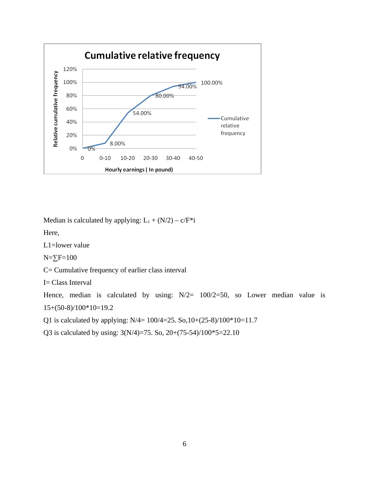
Median is calculated by applying: L1 + (N/2) – c/F*i
Here,
L1=lower value
N=∑F=100
C= Cumulative frequency of earlier class interval
I= Class Interval
Hence, median is calculated by using: N/2= 100/2=50, so Lower median value is
15+(50-8)/100*10=19.2
Q1 is calculated by applying: N/4= 100/4=25. So,10+(25-8)/100*10=11.7
Q3 is calculated by using: 3(N/4)=75. So, 20+(75-54)/100*5=22.10
6
⊘ This is a preview!⊘
Do you want full access?
Subscribe today to unlock all pages.
Trusted by 1+ million students worldwide
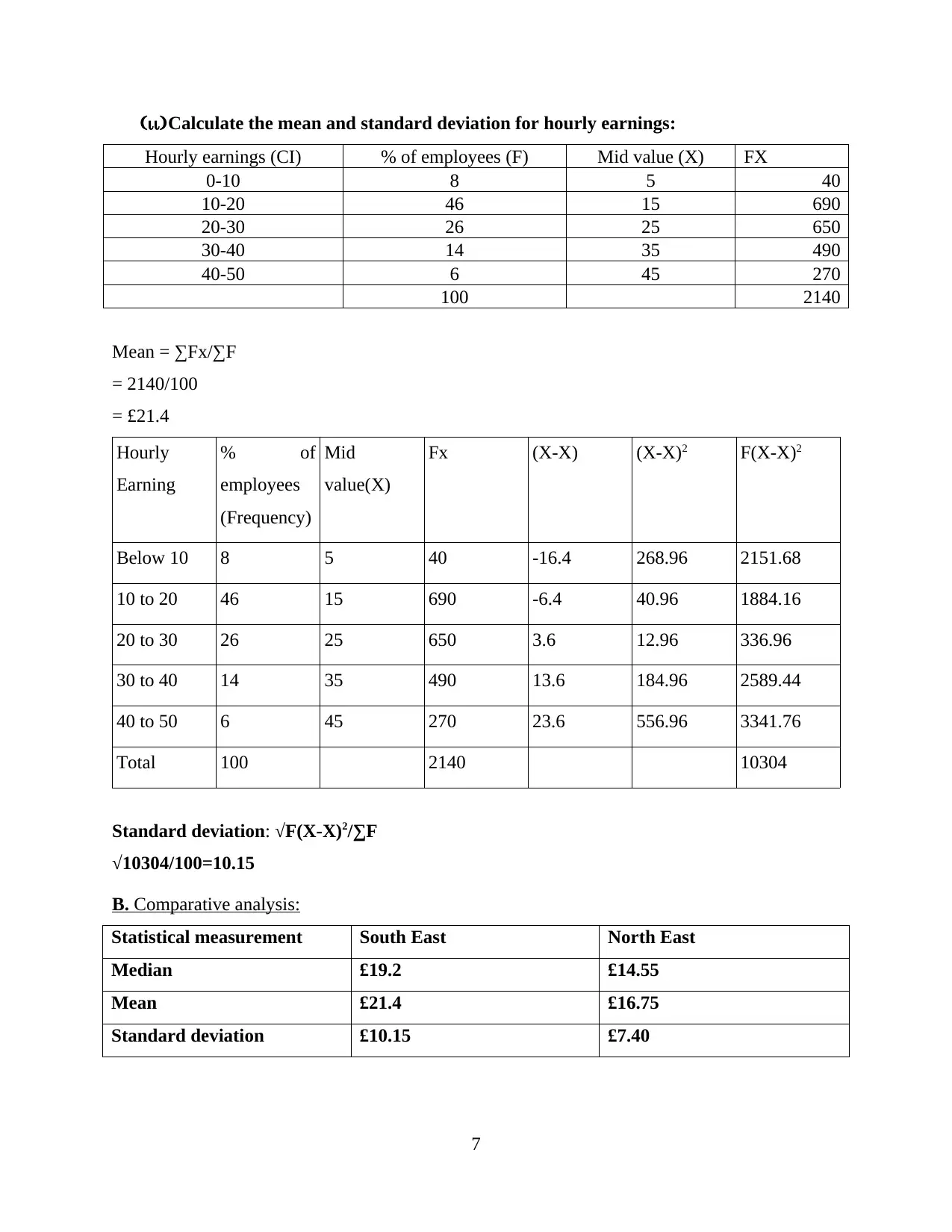
(ii)Calculate the mean and standard deviation for hourly earnings:
Hourly earnings (CI) % of employees (F) Mid value (X) FX
0-10 8 5 40
10-20 46 15 690
20-30 26 25 650
30-40 14 35 490
40-50 6 45 270
100 2140
Mean = ∑Fx/∑F
= 2140/100
= £21.4
Hourly
Earning
% of
employees
(Frequency)
Mid
value(X)
Fx (X-X) (X-X)2 F(X-X)2
Below 10 8 5 40 -16.4 268.96 2151.68
10 to 20 46 15 690 -6.4 40.96 1884.16
20 to 30 26 25 650 3.6 12.96 336.96
30 to 40 14 35 490 13.6 184.96 2589.44
40 to 50 6 45 270 23.6 556.96 3341.76
Total 100 2140 10304
Standard deviation: √F(X-X)2/∑F
√10304/100=10.15
B. Comparative analysis:
Statistical measurement South East North East
Median £19.2 £14.55
Mean £21.4 £16.75
Standard deviation £10.15 £7.40
7
Paraphrase This Document
Need a fresh take? Get an instant paraphrase of this document with our AI Paraphraser
As per the outcome, this is observed that in average of hourly earnings is found to £21.40 which
states that hourly earnings of South East health professionals does not match with the North East
is £16.75 which is less than the SE health candidates. On the other way, NE health candidates
have £14.55 which is lower than the SE health candidates. Although, in contrast, SE employee's
earnings demonstrates higher standard-deviation to £10.15 directing much variability.
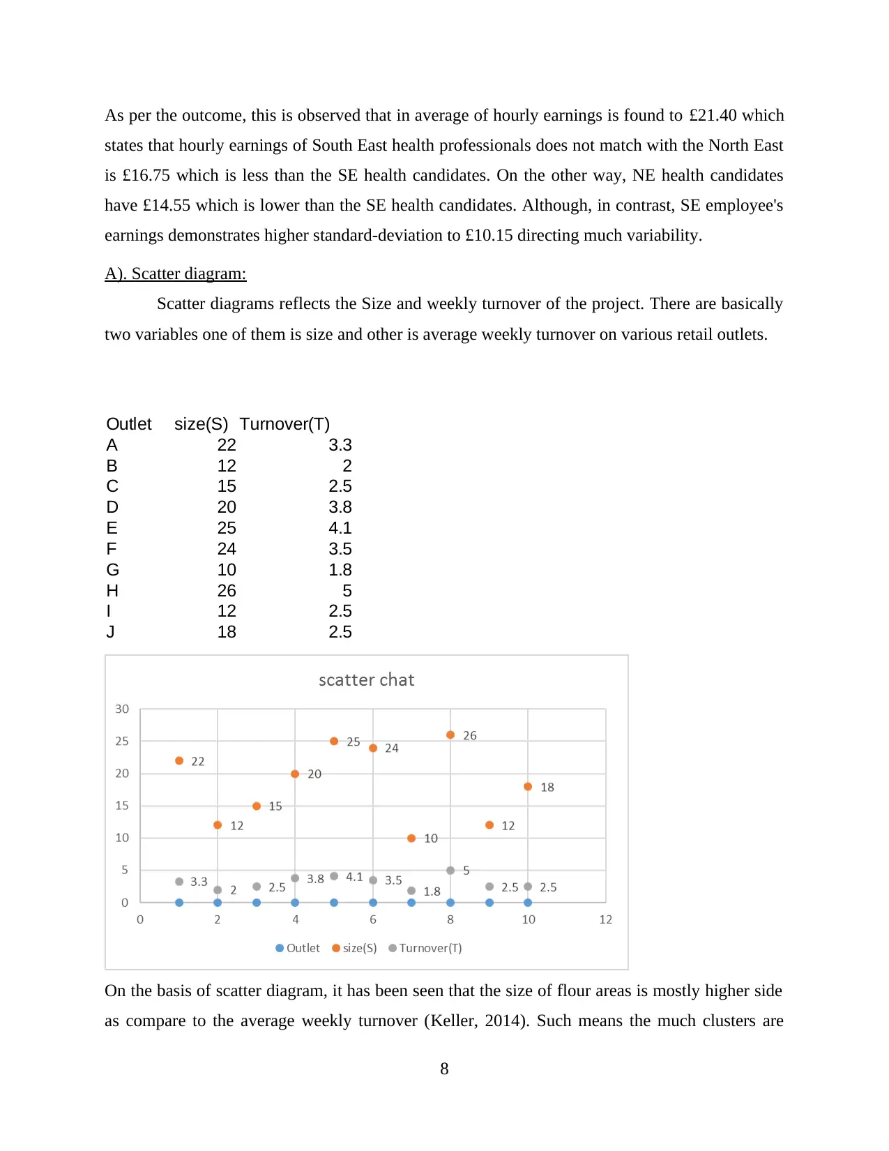
A). Scatter diagram:
Scatter diagrams reflects the Size and weekly turnover of the project. There are basically
two variables one of them is size and other is average weekly turnover on various retail outlets.
Outlet size(S) Turnover(T)
A 22 3.3
B 12 2
C 15 2.5
D 20 3.8
E 25 4.1
F 24 3.5
G 10 1.8
H 26 5
I 12 2.5
J 18 2.5
On the basis of scatter diagram, it has been seen that the size of flour areas is mostly higher side
as compare to the average weekly turnover (Keller, 2014). Such means the much clusters are
8
states that hourly earnings of South East health professionals does not match with the North East
is £16.75 which is less than the SE health candidates. On the other way, NE health candidates
have £14.55 which is lower than the SE health candidates. Although, in contrast, SE employee's
earnings demonstrates higher standard-deviation to £10.15 directing much variability.
A). Scatter diagram:
Scatter diagrams reflects the Size and weekly turnover of the project. There are basically
two variables one of them is size and other is average weekly turnover on various retail outlets.
Outlet size(S) Turnover(T)
A 22 3.3
B 12 2
C 15 2.5
D 20 3.8
E 25 4.1
F 24 3.5
G 10 1.8
H 26 5
I 12 2.5
J 18 2.5
On the basis of scatter diagram, it has been seen that the size of flour areas is mostly higher side
as compare to the average weekly turnover (Keller, 2014). Such means the much clusters are
8
observed Under the above mentioned graphs. The turnover is analyzed at the same level with
various sizes at the common point.
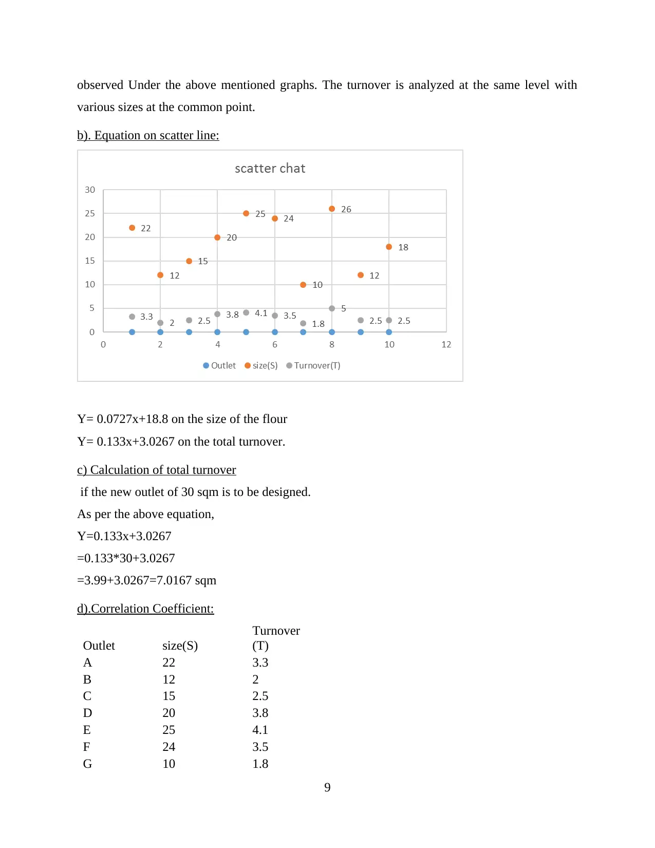
b). Equation on scatter line:
Y= 0.0727x+18.8 on the size of the flour
Y= 0.133x+3.0267 on the total turnover.
c) Calculation of total turnover
if the new outlet of 30 sqm is to be designed.
As per the above equation,
Y=0.133x+3.0267
=0.133*30+3.0267
=3.99+3.0267=7.0167 sqm
d).Correlation Coefficient:
Outlet size(S)
Turnover
(T)
A 22 3.3
B 12 2
C 15 2.5
D 20 3.8
E 25 4.1
F 24 3.5
G 10 1.8
9
various sizes at the common point.
b). Equation on scatter line:
Y= 0.0727x+18.8 on the size of the flour
Y= 0.133x+3.0267 on the total turnover.
c) Calculation of total turnover
if the new outlet of 30 sqm is to be designed.
As per the above equation,
Y=0.133x+3.0267
=0.133*30+3.0267
=3.99+3.0267=7.0167 sqm
d).Correlation Coefficient:
Outlet size(S)
Turnover
(T)
A 22 3.3
B 12 2
C 15 2.5
D 20 3.8
E 25 4.1
F 24 3.5
G 10 1.8
9
⊘ This is a preview!⊘
Do you want full access?
Subscribe today to unlock all pages.
Trusted by 1+ million students worldwide
1 out of 18
Related Documents


Your All-in-One AI-Powered Toolkit for Academic Success.
+13062052269
info@desklib.com
Available 24*7 on WhatsApp / Email
![[object Object]](/_next/static/media/star-bottom.7253800d.svg)
Unlock your academic potential
Copyright © 2020–2026 A2Z Services. All Rights Reserved. Developed and managed by ZUCOL.