Statistical Computing (STAT878) Assignment 1: Comprehensive Analysis

This document presents a comprehensive solution to Assignment 1 for the STAT878 Statistical Computing course. The solution addresses three key areas: Maximum Likelihood Estimation (MLE) using the Newton-Raphson method, Bayesian statistics with posterior plot estimation, and Ridge Regression. The MLE section includes model definition, variable identification, and probabilistic relationships, along with code implementation. The Bayesian statistics component focuses on plotting posterior estimates using Monte Carlo simulations. The Ridge Regression section involves loading data, plotting predictor variables, calculating correlations, and computing coefficient estimates with ridge parameters, along with graphical representations of the results. The assignment leverages statistical techniques to analyze and model data related to train cancellations, temperature, and rainfall.

UNIVERSITY AFFILIATION
FACULTY OR DEPARTMENT
STAT878: STATISTICAL COMPUTING
TITLE:
ASSIGNMENT I
STUDENT NAME:
STUDENT REGISTRATION NUMBER:
PROFESSOR (TUTOR)
DATE OF SUBMISSION

1
QUESTION 1: MLE WITH NEWTON-RAPHSON (21 marks)
Part A: Statistical Model
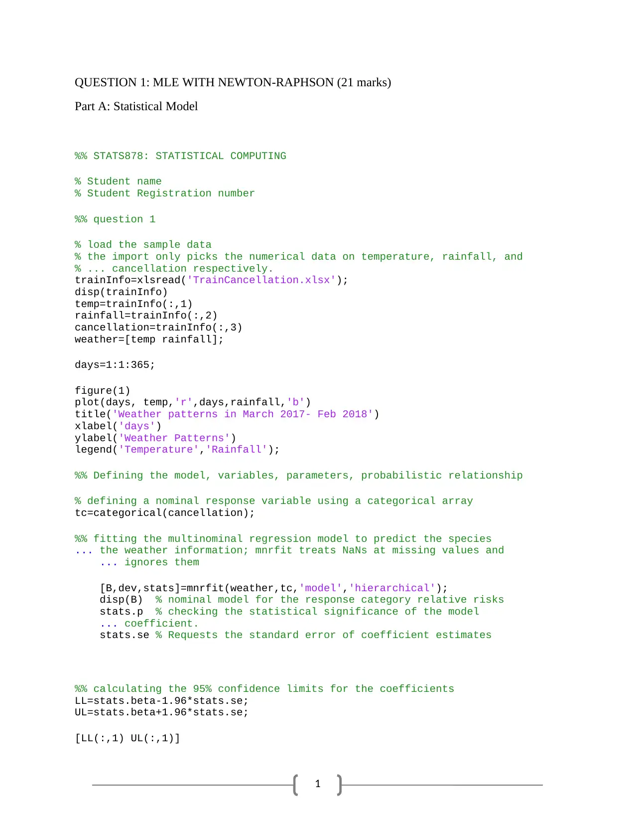
%% STATS878: STATISTICAL COMPUTING
% Student name
% Student Registration number
%% question 1
% load the sample data
% the import only picks the numerical data on temperature, rainfall, and
% ... cancellation respectively.
trainInfo=xlsread('TrainCancellation.xlsx');
disp(trainInfo)
temp=trainInfo(:,1)
rainfall=trainInfo(:,2)
cancellation=trainInfo(:,3)
weather=[temp rainfall];
days=1:1:365;
figure(1)
plot(days, temp,'r',days,rainfall,'b')
title('Weather patterns in March 2017- Feb 2018')
xlabel('days')
ylabel('Weather Patterns')
legend('Temperature','Rainfall');
%% Defining the model, variables, parameters, probabilistic relationship
% defining a nominal response variable using a categorical array
tc=categorical(cancellation);
%% fitting the multinominal regression model to predict the species
... the weather information; mnrfit treats NaNs at missing values and
... ignores them
[B,dev,stats]=mnrfit(weather,tc,'model','hierarchical');
disp(B) % nominal model for the response category relative risks
stats.p % checking the statistical significance of the model
... coefficient.
stats.se % Requests the standard error of coefficient estimates
%% calculating the 95% confidence limits for the coefficients
LL=stats.beta-1.96*stats.se;
UL=stats.beta+1.96*stats.se;
[LL(:,1) UL(:,1)]

2
figure(2)
plot(days,cancellation)
[R,M,B]=regression(temp,cancellation)
figure (3)
plotregression(temp,cancellation)
[s,c,r,d]=regr(temp,cancellation,1,2)
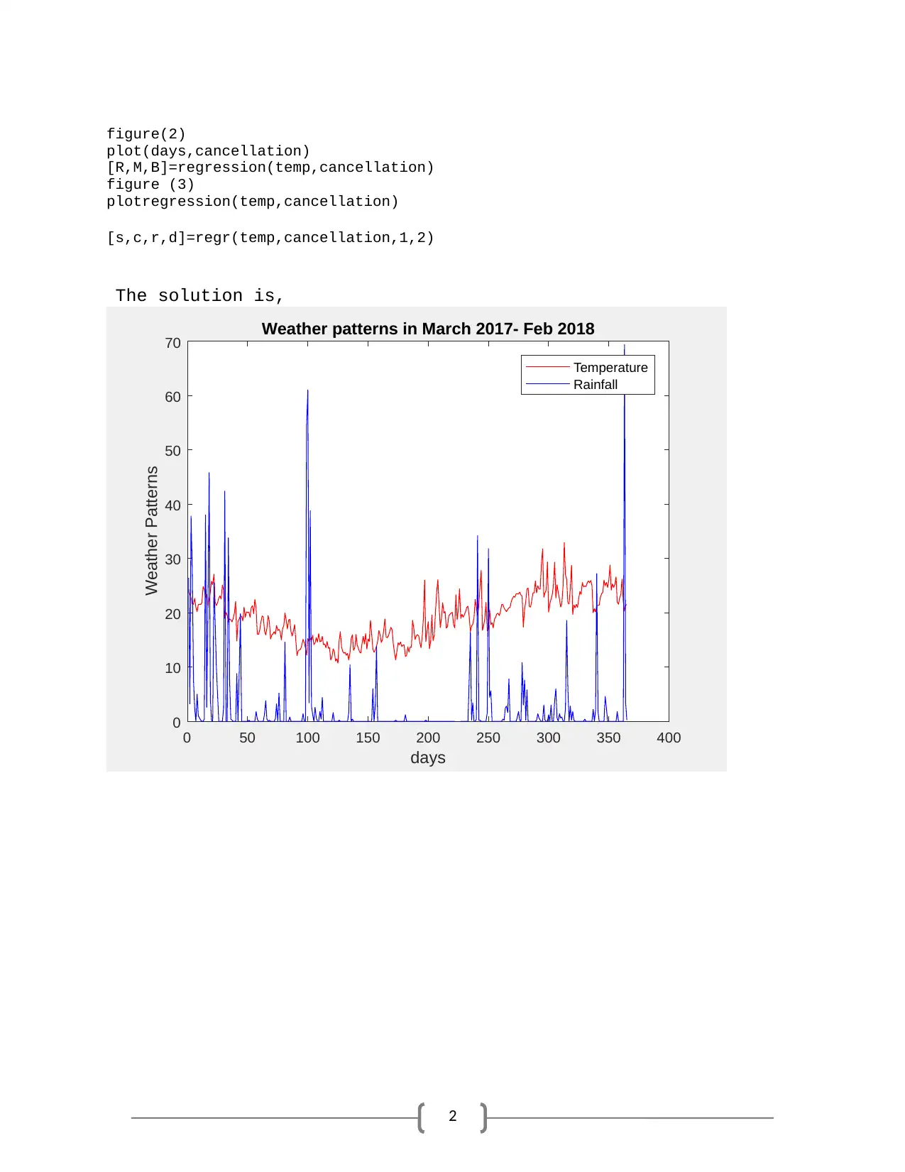
The solution is,
0 50 100 150 200 250 300 350 400
days
0
10
20
30
40
50
60
70
Weather Patterns
Weather patterns in March 2017- Feb 2018
Temperature
Rainfall

3
0 5 10 15 20 25 30
Target
0
5
10
15
20
25
30
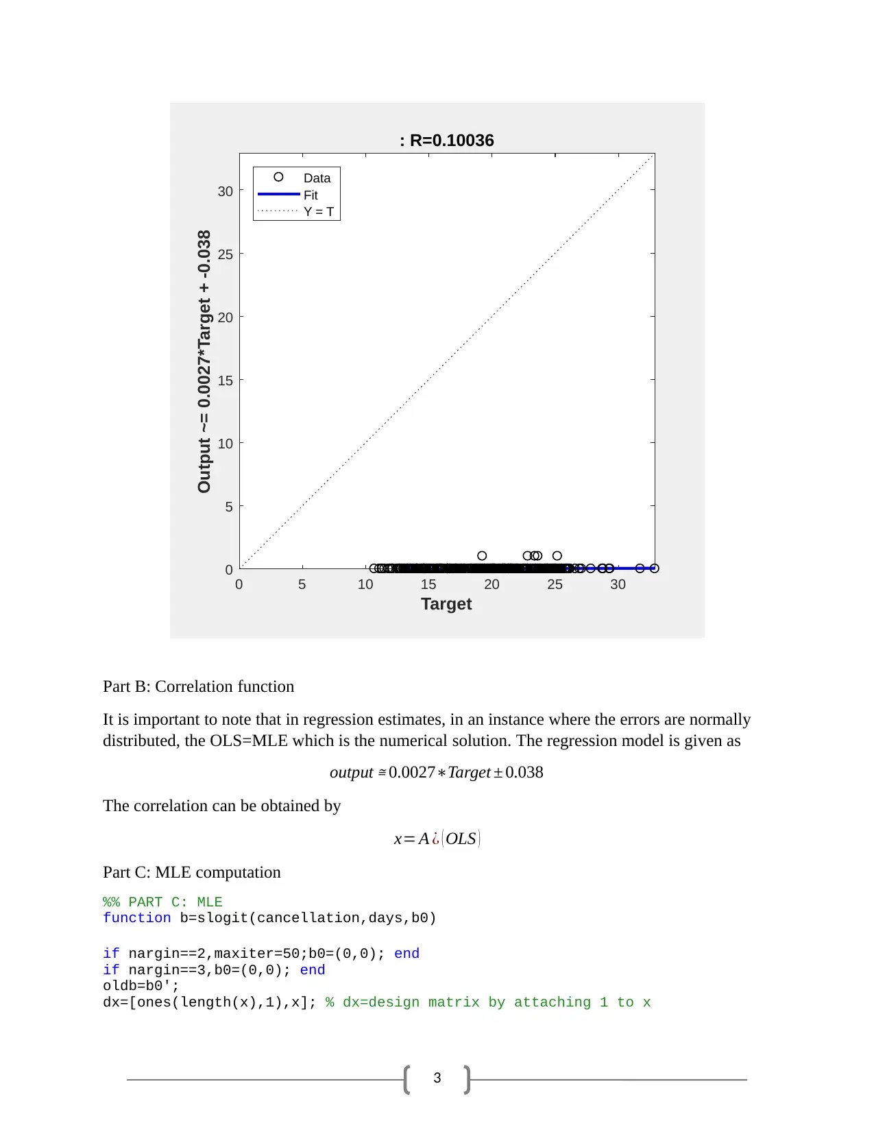
Output ~= 0.0027*Target + -0.038
: R=0.10036
Data
Fit
Y = T
Part B: Correlation function
It is important to note that in regression estimates, in an instance where the errors are normally
distributed, the OLS=MLE which is the numerical solution. The regression model is given as
output ≅ 0.0027∗Target ± 0.038
The correlation can be obtained by
x= A ¿ ( OLS )
Part C: MLE computation
%% PART C: MLE
function b=slogit(cancellation,days,b0)
if nargin==2,maxiter=50;b0=(0,0); end
if nargin==3,b0=(0,0); end
oldb=b0';
dx=[ones(length(x),1),x]; % dx=design matrix by attaching 1 to x

4
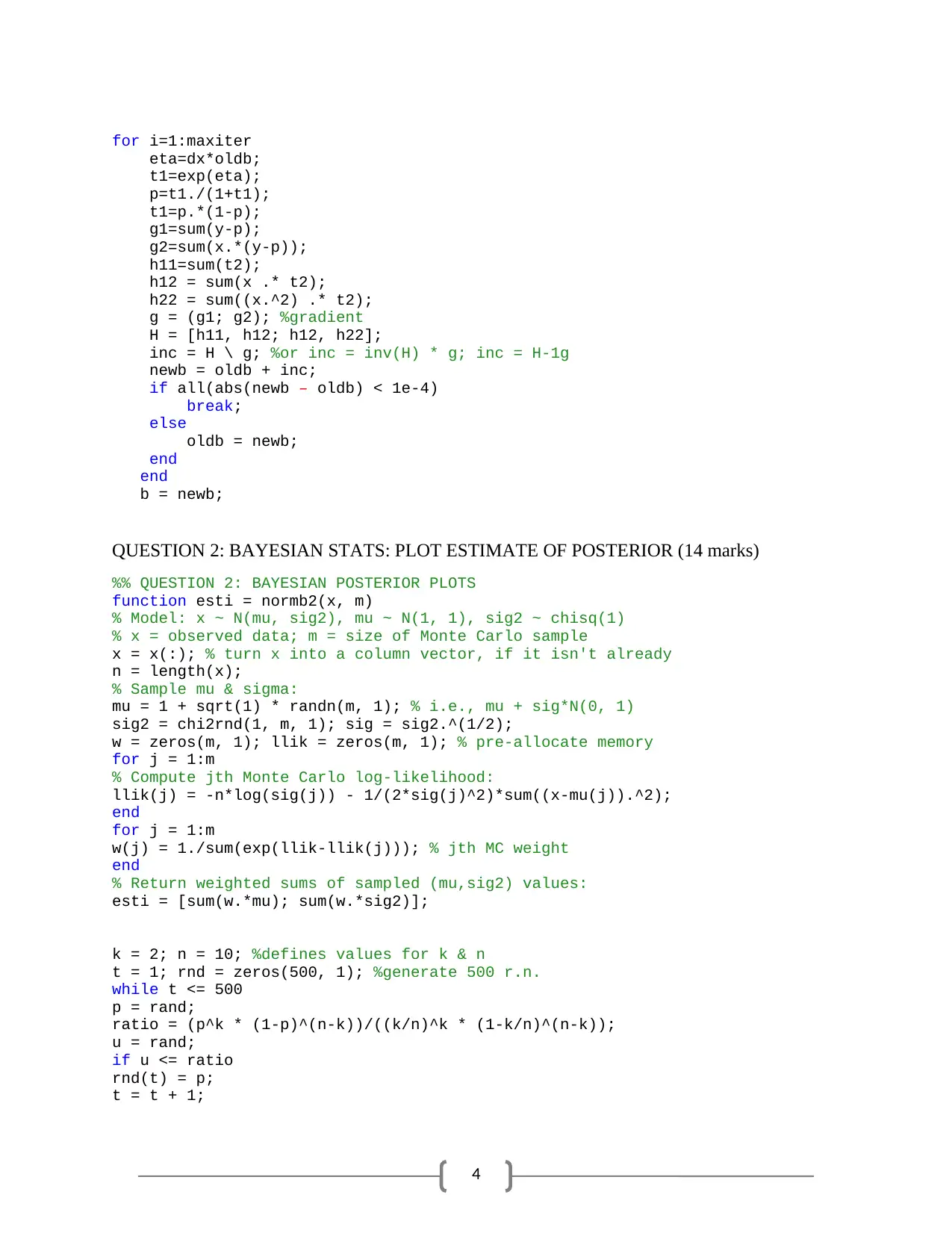
for i=1:maxiter
eta=dx*oldb;
t1=exp(eta);
p=t1./(1+t1);
t1=p.*(1-p);
g1=sum(y-p);
g2=sum(x.*(y-p));
h11=sum(t2);
h12 = sum(x .* t2);
h22 = sum((x.^2) .* t2);
g = (g1; g2); %gradient
H = [h11, h12; h12, h22];
inc = H \ g; %or inc = inv(H) * g; inc = H-1g
newb = oldb + inc;
if all(abs(newb – oldb) < 1e-4)
break;
else
oldb = newb;
end
end
b = newb;
QUESTION 2: BAYESIAN STATS: PLOT ESTIMATE OF POSTERIOR (14 marks)
%% QUESTION 2: BAYESIAN POSTERIOR PLOTS
function esti = normb2(x, m)
% Model: x ~ N(mu, sig2), mu ~ N(1, 1), sig2 ~ chisq(1)
% x = observed data; m = size of Monte Carlo sample
x = x(:); % turn x into a column vector, if it isn't already
n = length(x);
% Sample mu & sigma:
mu = 1 + sqrt(1) * randn(m, 1); % i.e., mu + sig*N(0, 1)
sig2 = chi2rnd(1, m, 1); sig = sig2.^(1/2);
w = zeros(m, 1); llik = zeros(m, 1); % pre-allocate memory
for j = 1:m
% Compute jth Monte Carlo log-likelihood:
llik(j) = -n*log(sig(j)) - 1/(2*sig(j)^2)*sum((x-mu(j)).^2);
end
for j = 1:m
w(j) = 1./sum(exp(llik-llik(j))); % jth MC weight
end
% Return weighted sums of sampled (mu,sig2) values:
esti = [sum(w.*mu); sum(w.*sig2)];
k = 2; n = 10; %defines values for k & n
t = 1; rnd = zeros(500, 1); %generate 500 r.n.
while t <= 500
p = rand;
ratio = (p^k * (1-p)^(n-k))/((k/n)^k * (1-k/n)^(n-k));
u = rand;
if u <= ratio
rnd(t) = p;
t = t + 1;

5
end
end
x = 0:0.01:1;
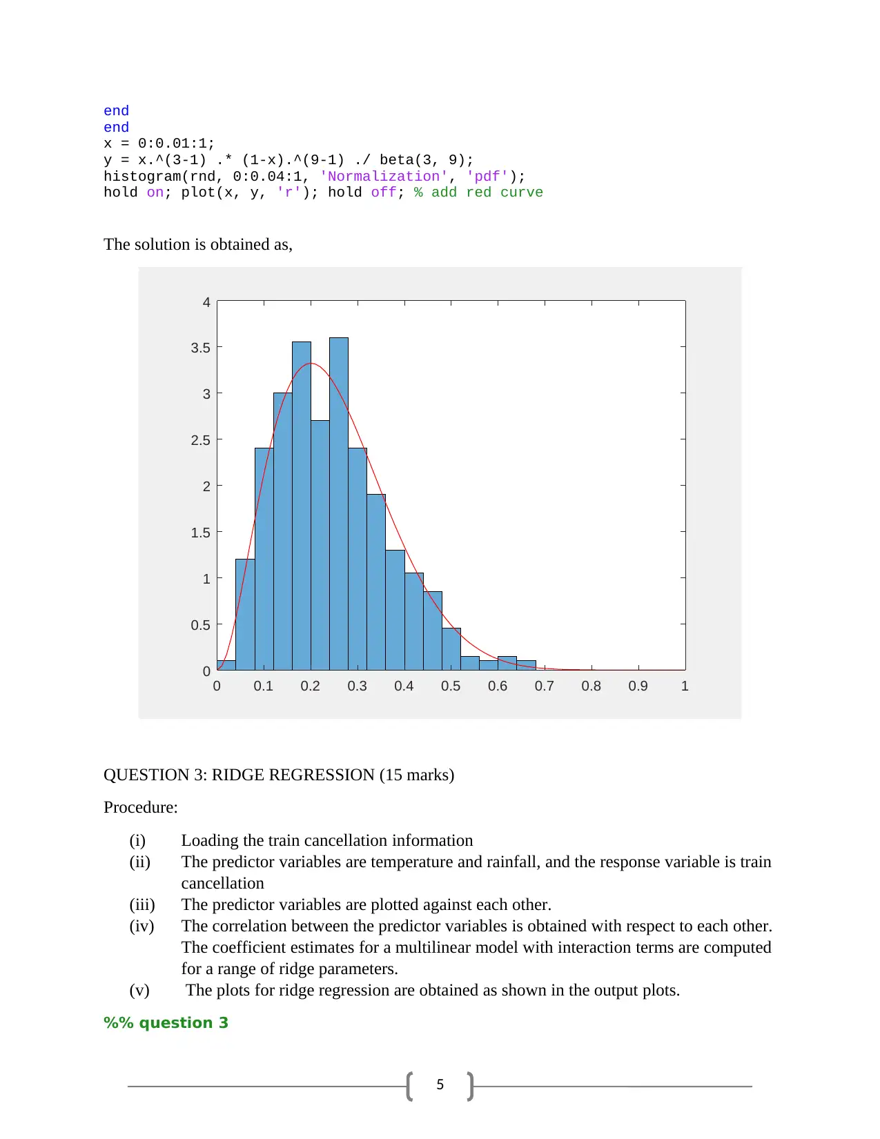
y = x.^(3-1) .* (1-x).^(9-1) ./ beta(3, 9);
histogram(rnd, 0:0.04:1, 'Normalization', 'pdf');
hold on; plot(x, y, 'r'); hold off; % add red curve
The solution is obtained as,
0 0.1 0.2 0.3 0.4 0.5 0.6 0.7 0.8 0.9 1
0
0.5
1
1.5
2
2.5
3
3.5
4
QUESTION 3: RIDGE REGRESSION (15 marks)
Procedure:
(i) Loading the train cancellation information
(ii) The predictor variables are temperature and rainfall, and the response variable is train
cancellation
(iii) The predictor variables are plotted against each other.
(iv) The correlation between the predictor variables is obtained with respect to each other.
The coefficient estimates for a multilinear model with interaction terms are computed
for a range of ridge parameters.
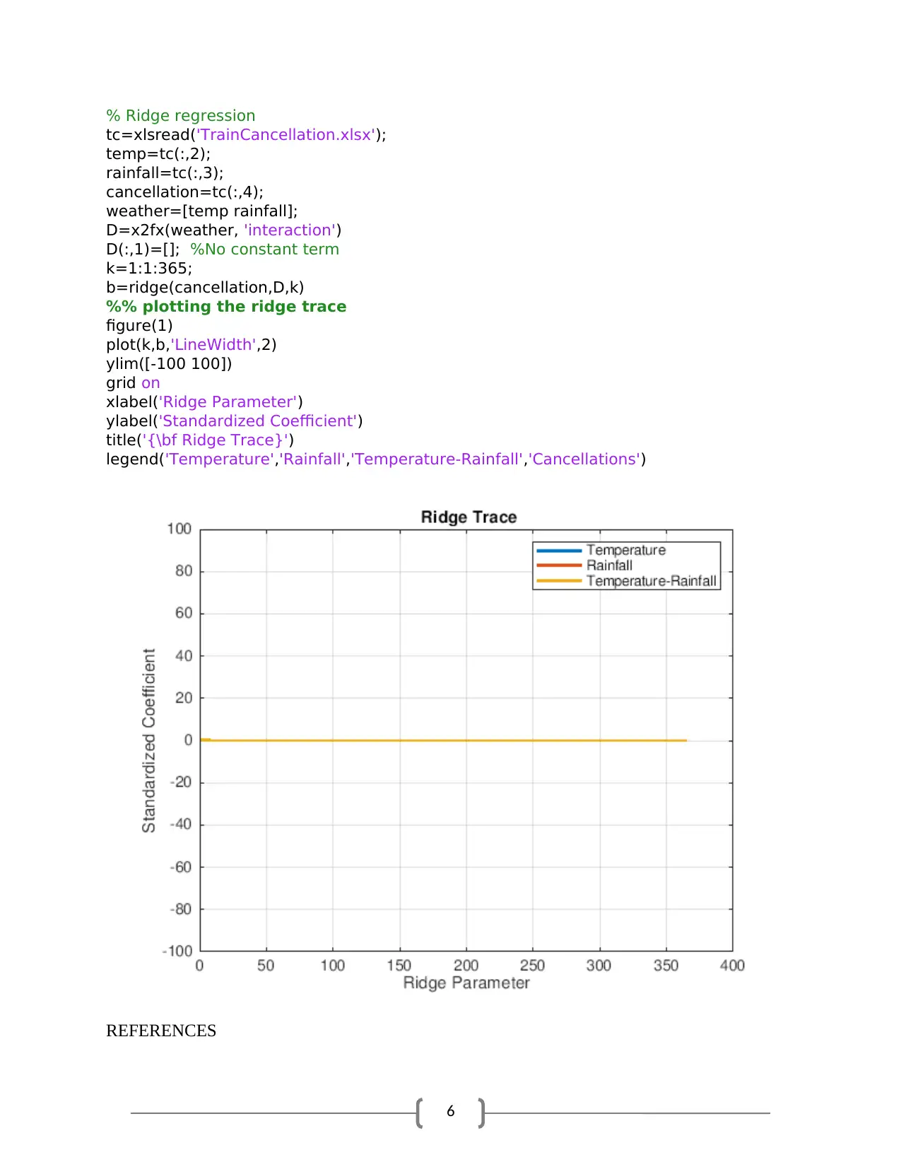
(v) The plots for ridge regression are obtained as shown in the output plots.
%% question 3

6
% Ridge regression
tc=xlsread('TrainCancellation.xlsx');
temp=tc(:,2);
rainfall=tc(:,3);
cancellation=tc(:,4);
weather=[temp rainfall];
D=x2fx(weather, 'interaction')
D(:,1)=[]; %No constant term
k=1:1:365;
b=ridge(cancellation,D,k)
%% plotting the ridge trace
figure(1)
plot(k,b,'LineWidth',2)
ylim([-100 100])
grid on
xlabel('Ridge Parameter')
ylabel('Standardized Coefficient')
title('{\bf Ridge Trace}')
legend('Temperature','Rainfall','Temperature-Rainfall','Cancellations')
REFERENCES

7
[1] Dobson, A. J., and A. G. Barnett. An Introduction to Generalized Linear Models. Chapman
and Hall/CRC. Taylor & Francis Group, 2008.
[2] K. Sigmon and T. A. Davis, MATLAB Primer, Sixth Edition, Chapman and
Hall/CRC, Boca Raton, FL, 2002
[3] Marquardt, D.W. “Generalized Inverses, Ridge Regression, Biased Linear Estimation, and
Nonlinear Estimation.” Technometrics. Vol. 12, No. 3, 1970, pp. 591–612.