Statistical Analysis of County Crime: Report and Findings

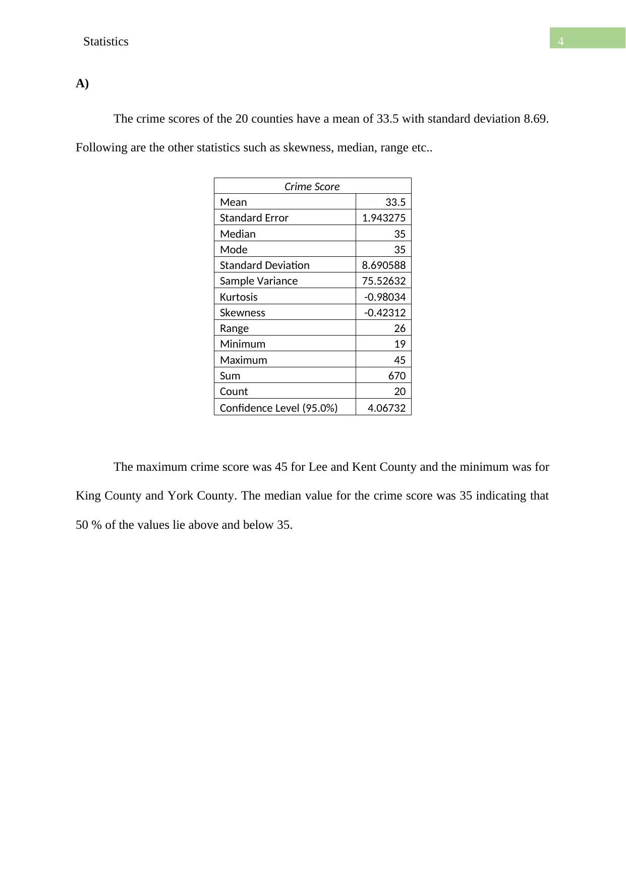
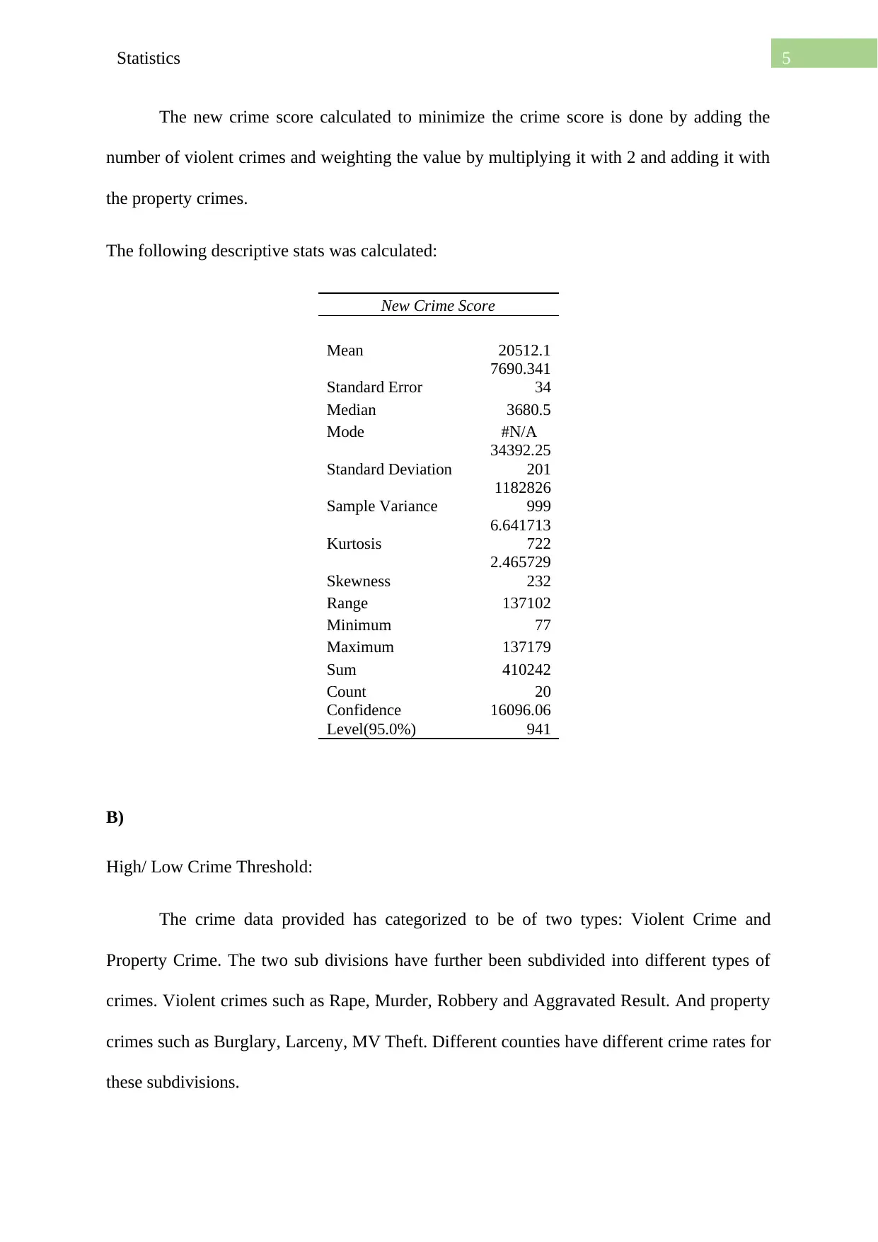
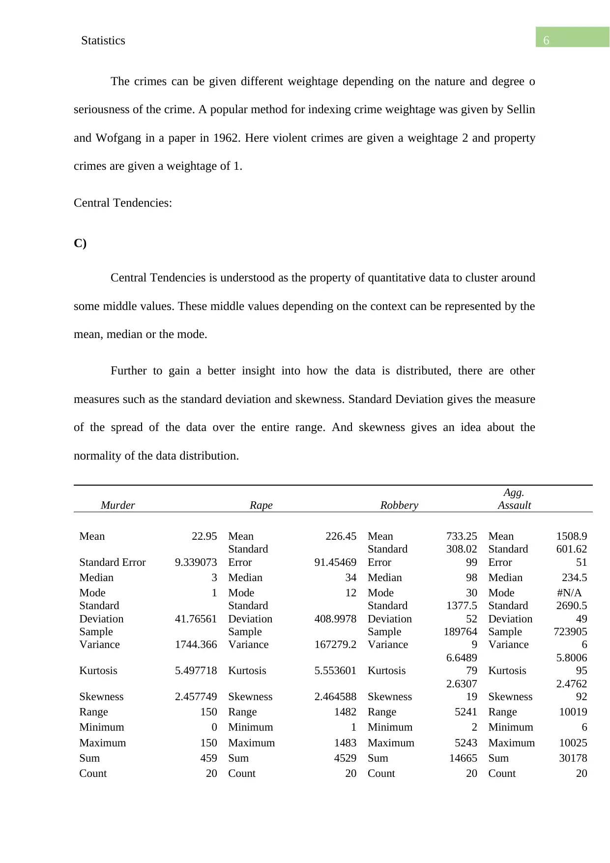
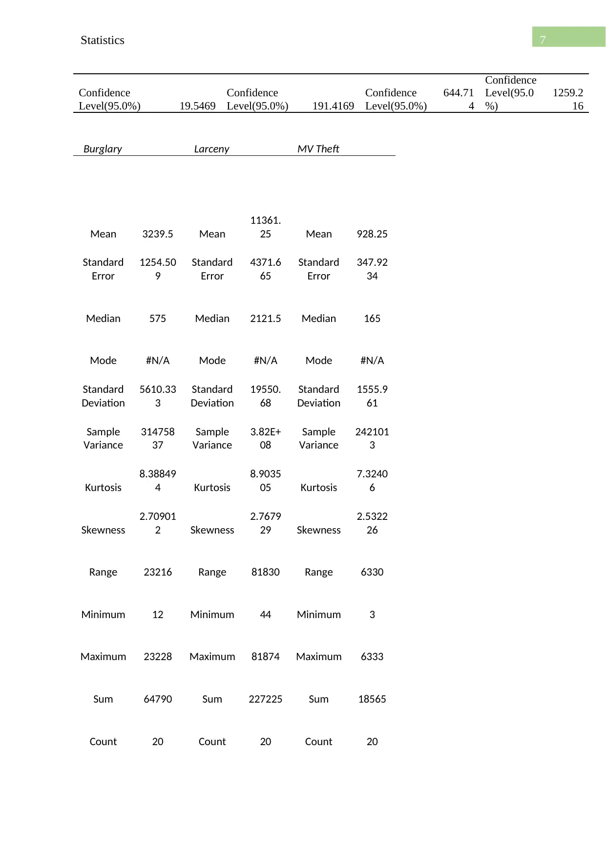
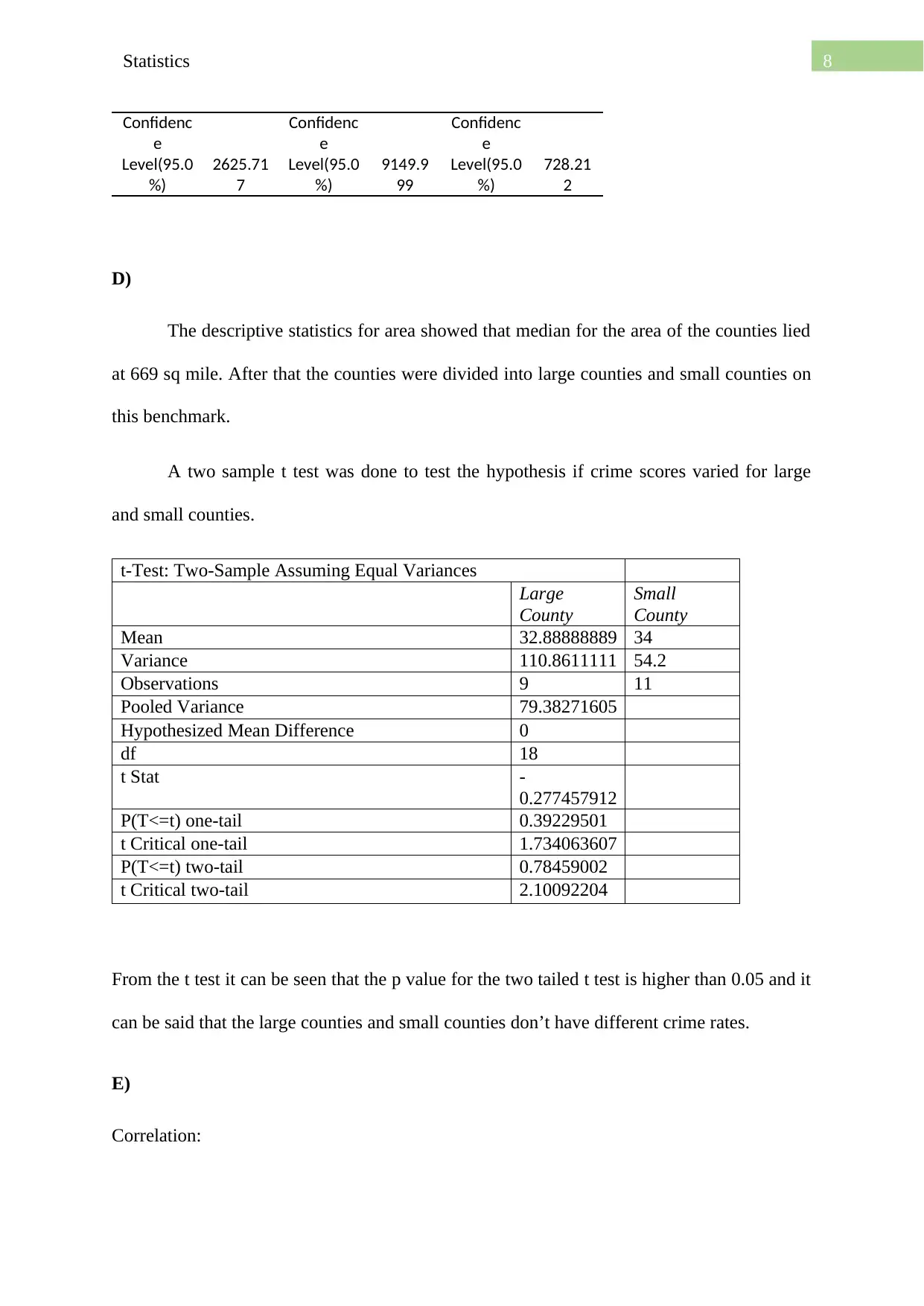
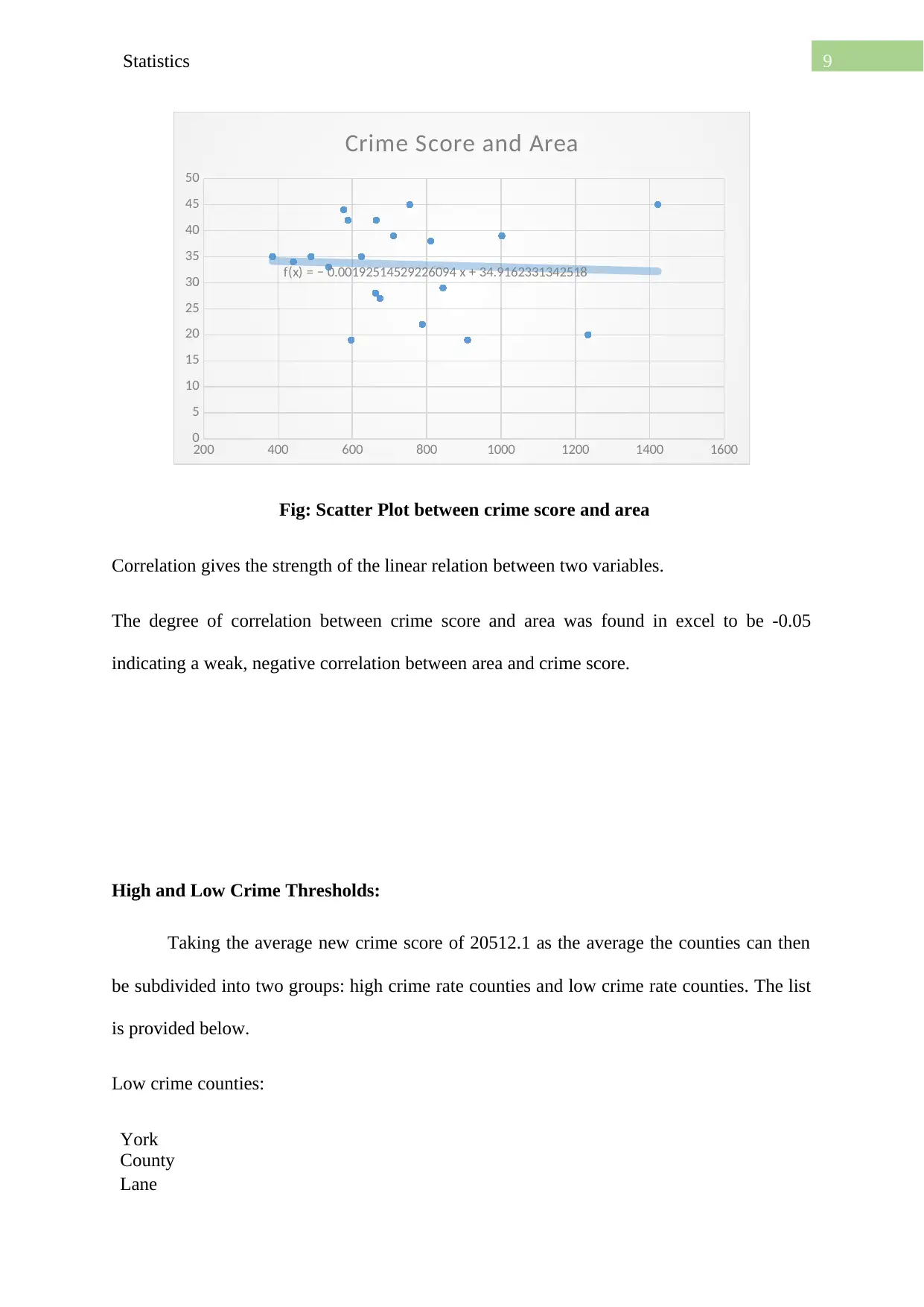
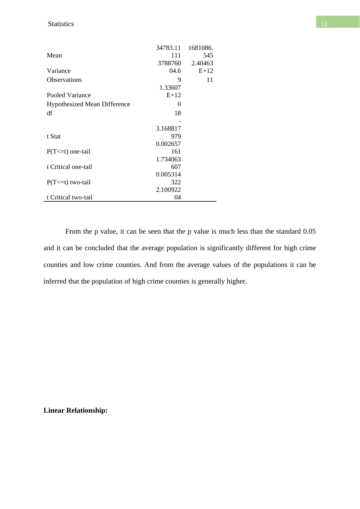
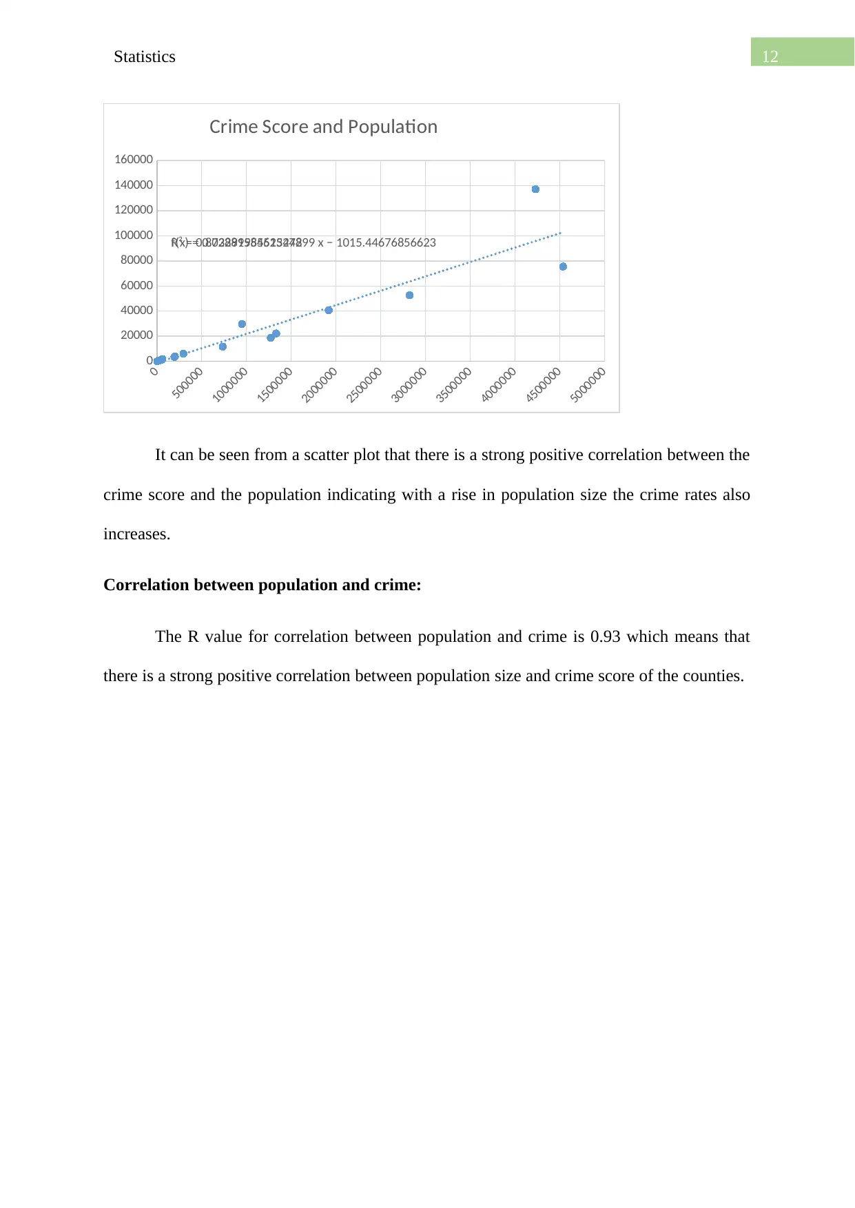
This report provides a statistical analysis of county crime data, addressing both descriptive and inferential statistics to understand crime patterns. The report begins with conceptual and operational definitions of crime, followed by a descriptive statistical analysis of crime scores, including mean, media...Read More

Running head: Statistics
Statistics
Name of the Student
Name of the University

2Statistics
Table of Contents
Introduction:...............................................................................................................................3
A)................................................................................................................................................4
B)................................................................................................................................................5
C)................................................................................................................................................6
D)................................................................................................................................................7
E)................................................................................................................................................8
High and Low Crime Thresholds:..............................................................................................9
Inferential Statistics:.................................................................................................................10
References:...............................................................................................................................12

3Statistics
Introduction:
Conceptual Definition of Crime:
Generally speaking crime is understood to be any unlawful act punishable by a state
or any established authority. In current criminal law, there is not an agreed upon definition of
crime. A crime can change depending upon the context. It has been seen that acts that were
considered as crime in the past may not be considered as crime now. Crime is also cultural
and the geographical region and its unique culture may have different idea of what is crime
and what is not crime. Another common definition is that a crime or criminal offense is an
action that is not only harmful to an individual or a group of individual but also at large to a
community, society or the state.
Operational definition of crime:
An act is a crime, if it is declared as such by the relevant state or authorities. An
operational definition of crime can be said to be the laid down laws for the well-being of a
society in a region and the violation of the said law. The relevant authorities then intervene to
check the law breakers and bring them to justice.

4Statistics
A)
The crime scores of the 20 counties have a mean of 33.5 with standard deviation 8.69.
Following are the other statistics such as skewness, median, range etc..
Crime Score
Mean 33.5
Standard Error 1.943275
Median 35
Mode 35
Standard Deviation 8.690588
Sample Variance 75.52632
Kurtosis -0.98034
Skewness -0.42312
Range 26
Minimum 19
Maximum 45
Sum 670
Count 20
Confidence Level (95.0%) 4.06732
The maximum crime score was 45 for Lee and Kent County and the minimum was for
King County and York County. The median value for the crime score was 35 indicating that
50 % of the values lie above and below 35.

5Statistics
The new crime score calculated to minimize the crime score is done by adding the
number of violent crimes and weighting the value by multiplying it with 2 and adding it with
the property crimes.
The following descriptive stats was calculated:
New Crime Score
Mean 20512.1
Standard Error
7690.341
34
Median 3680.5
Mode #N/A
Standard Deviation
34392.25
201
Sample Variance
1182826
999
Kurtosis
6.641713
722
Skewness
2.465729
232
Range 137102
Minimum 77
Maximum 137179
Sum 410242
Count 20
Confidence
Level(95.0%)
16096.06
941
B)
High/ Low Crime Threshold:
The crime data provided has categorized to be of two types: Violent Crime and
Property Crime. The two sub divisions have further been subdivided into different types of
crimes. Violent crimes such as Rape, Murder, Robbery and Aggravated Result. And property
crimes such as Burglary, Larceny, MV Theft. Different counties have different crime rates for
these subdivisions.

6Statistics
The crimes can be given different weightage depending on the nature and degree o
seriousness of the crime. A popular method for indexing crime weightage was given by Sellin
and Wofgang in a paper in 1962. Here violent crimes are given a weightage 2 and property
crimes are given a weightage of 1.
Central Tendencies:
C)
Central Tendencies is understood as the property of quantitative data to cluster around
some middle values. These middle values depending on the context can be represented by the
mean, median or the mode.
Further to gain a better insight into how the data is distributed, there are other
measures such as the standard deviation and skewness. Standard Deviation gives the measure
of the spread of the data over the entire range. And skewness gives an idea about the
normality of the data distribution.
Murder Rape Robbery
Agg.
Assault
Mean 22.95 Mean 226.45 Mean 733.25 Mean 1508.9
Standard Error 9.339073
Standard
Error 91.45469
Standard
Error
308.02
99
Standard
Error
601.62
51
Median 3 Median 34 Median 98 Median 234.5
Mode 1 Mode 12 Mode 30 Mode #N/A
Standard
Deviation 41.76561
Standard
Deviation 408.9978
Standard
Deviation
1377.5
52
Standard
Deviation
2690.5
49
Sample
Variance 1744.366
Sample
Variance 167279.2
Sample
Variance
189764
9
Sample
Variance
723905
6
Kurtosis 5.497718 Kurtosis 5.553601 Kurtosis
6.6489
79 Kurtosis
5.8006
95
Skewness 2.457749 Skewness 2.464588 Skewness
2.6307
19 Skewness
2.4762
92
Range 150 Range 1482 Range 5241 Range 10019
Minimum 0 Minimum 1 Minimum 2 Minimum 6
Maximum 150 Maximum 1483 Maximum 5243 Maximum 10025
Sum 459 Sum 4529 Sum 14665 Sum 30178
Count 20 Count 20 Count 20 Count 20

7Statistics
Confidence
Level(95.0%) 19.5469
Confidence
Level(95.0%) 191.4169
Confidence
Level(95.0%)
644.71
4
Confidence
Level(95.0
%)
1259.2
16
Burglary Larceny MV Theft
Mean 3239.5 Mean
11361.
25 Mean 928.25
Standard
Error
1254.50
9
Standard
Error
4371.6
65
Standard
Error
347.92
34
Median 575 Median 2121.5 Median 165
Mode #N/A Mode #N/A Mode #N/A
Standard
Deviation
5610.33
3
Standard
Deviation
19550.
68
Standard
Deviation
1555.9
61
Sample
Variance
314758
37
Sample
Variance
3.82E+
08
Sample
Variance
242101
3
Kurtosis
8.38849
4 Kurtosis
8.9035
05 Kurtosis
7.3240
6
Skewness
2.70901
2 Skewness
2.7679
29 Skewness
2.5322
26
Range 23216 Range 81830 Range 6330
Minimum 12 Minimum 44 Minimum 3
Maximum 23228 Maximum 81874 Maximum 6333
Sum 64790 Sum 227225 Sum 18565
Count 20 Count 20 Count 20

8Statistics
Confidenc
e
Level(95.0
%)
2625.71
7
Confidenc
e
Level(95.0
%)
9149.9
99
Confidenc
e
Level(95.0
%)
728.21
2
D)
The descriptive statistics for area showed that median for the area of the counties lied
at 669 sq mile. After that the counties were divided into large counties and small counties on
this benchmark.
A two sample t test was done to test the hypothesis if crime scores varied for large
and small counties.
t-Test: Two-Sample Assuming Equal Variances
Large
County
Small
County
Mean 32.88888889 34
Variance 110.8611111 54.2
Observations 9 11
Pooled Variance 79.38271605
Hypothesized Mean Difference 0
df 18
t Stat -
0.277457912
P(T<=t) one-tail 0.39229501
t Critical one-tail 1.734063607
P(T<=t) two-tail 0.78459002
t Critical two-tail 2.10092204
From the t test it can be seen that the p value for the two tailed t test is higher than 0.05 and it
can be said that the large counties and small counties don’t have different crime rates.
E)
Correlation:

9Statistics
200 400 600 800 1000 1200 1400 1600
0
5
10
15
20
25
30
35
40
45
50
f(x) = − 0.00192514529226094 x + 34.9162331342518
Crime Score and Area
Fig: Scatter Plot between crime score and area
Correlation gives the strength of the linear relation between two variables.
The degree of correlation between crime score and area was found in excel to be -0.05
indicating a weak, negative correlation between area and crime score.
High and Low Crime Thresholds:
Taking the average new crime score of 20512.1 as the average the counties can then
be subdivided into two groups: high crime rate counties and low crime rate counties. The list
is provided below.
Low crime counties:
York
County
Lane

10Statistics
County
Ida County
Bell County
Kent County
Webb
County
Kern
County
Kane
County
Cook
County
High crime counties:
Jay County
Ray County
King
County
Nye County
Bay County
Cass County
Pike County
Knox
County
Clay County
Lake
County
Lee County
Inferential Statistics:
To check the hypothesis that population is a key indicator of high crime counties and
low crime counties, a two sample t test is done to check if the average population is different
for both the categories.
t-Test: Two-Sample Assuming Equal Variances
Low
Crime
High
Crime

11Statistics
Mean
34783.11
111
1681086.
545
Variance
3788760
04.6
2.40463
E+12
Observations 9 11
Pooled Variance
1.33607
E+12
Hypothesized Mean Difference 0
df 18
t Stat
-
3.168817
979
P(T<=t) one-tail
0.002657
161
t Critical one-tail
1.734063
607
P(T<=t) two-tail
0.005314
322
t Critical two-tail
2.100922
04
From the p value, it can be seen that the p value is much less than the standard 0.05
and it can be concluded that the average population is significantly different for high crime
counties and low crime counties. And from the average values of the populations it can be
inferred that the population of high crime counties is generally higher.
Linear Relationship:

12Statistics
0
500000
1000000
1500000
2000000
2500000
3000000
3500000
4000000
4500000
5000000
0
20000
40000
60000
80000
100000
120000
140000
160000
f(x) = 0.0228955562547899 x − 1015.44676856623R² = 0.873891984513242
Crime Score and Population
It can be seen from a scatter plot that there is a strong positive correlation between the
crime score and the population indicating with a rise in population size the crime rates also
increases.
Correlation between population and crime:
The R value for correlation between population and crime is 0.93 which means that
there is a strong positive correlation between population size and crime score of the counties.

13Statistics
References:
Allen, M., 2016. Police-reported crime statistics in Canada, 2015. Statistics Canada.
Buonanno, P., Drago, F., Galbiati, R. and Vertova, P., 2018. How much should we trust
crime statistics? A comparison between EU and US. European Journal of Law and
Economics, 46(3), pp.343-357.
Chen, W. and Keen, M., 2014. Does inequality increase crime? The effect of income
inequality on crime rates in California counties. Working Paper.
Edelman, P., 2019. Not a crime to be poor: The criminalization of poverty in America. The
New Press.
Falls, G.A. and Thompson, P.B., 2014. Casinos, casino size, and crime: A panel data analysis
of Michigan counties. The Quarterly Review of Economics and Finance, 54(1), pp.123-132.
Jensen, E., Center for Court Innovation and United States of America, 2015. Building a Safer
Tomorrow: A Process Evaluation of Grand Forks County's Defending Childhood Initiative.
Miles, T.J. and Cox, A.B., 2014. Does immigration enforcement reduce crime? evidence
from secure communities. The Journal of Law and Economics, 57(4), pp.937-973.
Monuteaux, M.C., Lee, L.K., Hemenway, D., Mannix, R. and Fleegler, E.W., 2015. Firearm
ownership and violent crime in the US: an ecologic study. American journal of preventive
medicine, 49(2), pp.207-214.
Raleigh, E. and Galster, G., 2015. Neighborhood disinvestment, abandonment, and crime
dynamics. Journal of Urban Affairs, 37(4), pp.367-396.
Sohn, D.W., 2016. Residential crimes and neighbourhood built environment: Assessing the
effectiveness of crime prevention through environmental design (CPTED). Cities, 52, pp.86-
93.