Quantitative Methods Report: Statistical Analysis of Business Data

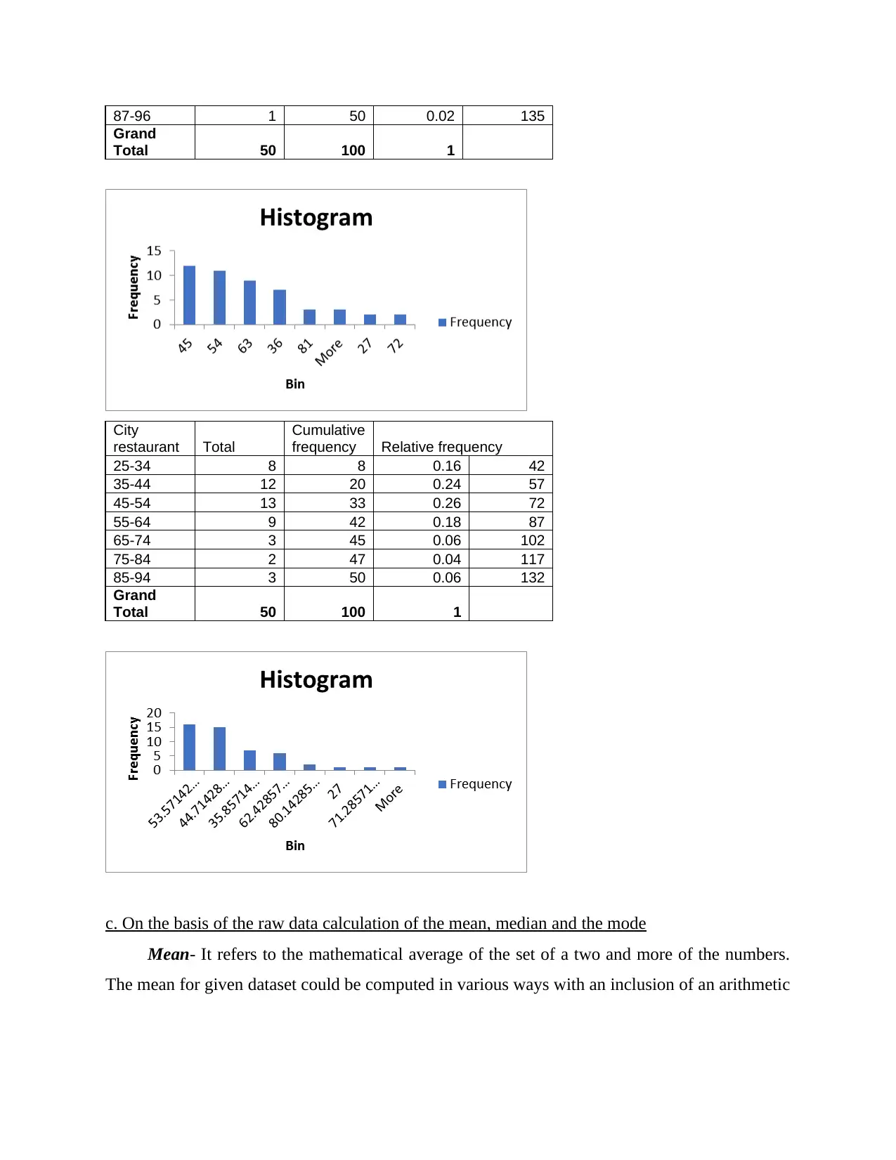
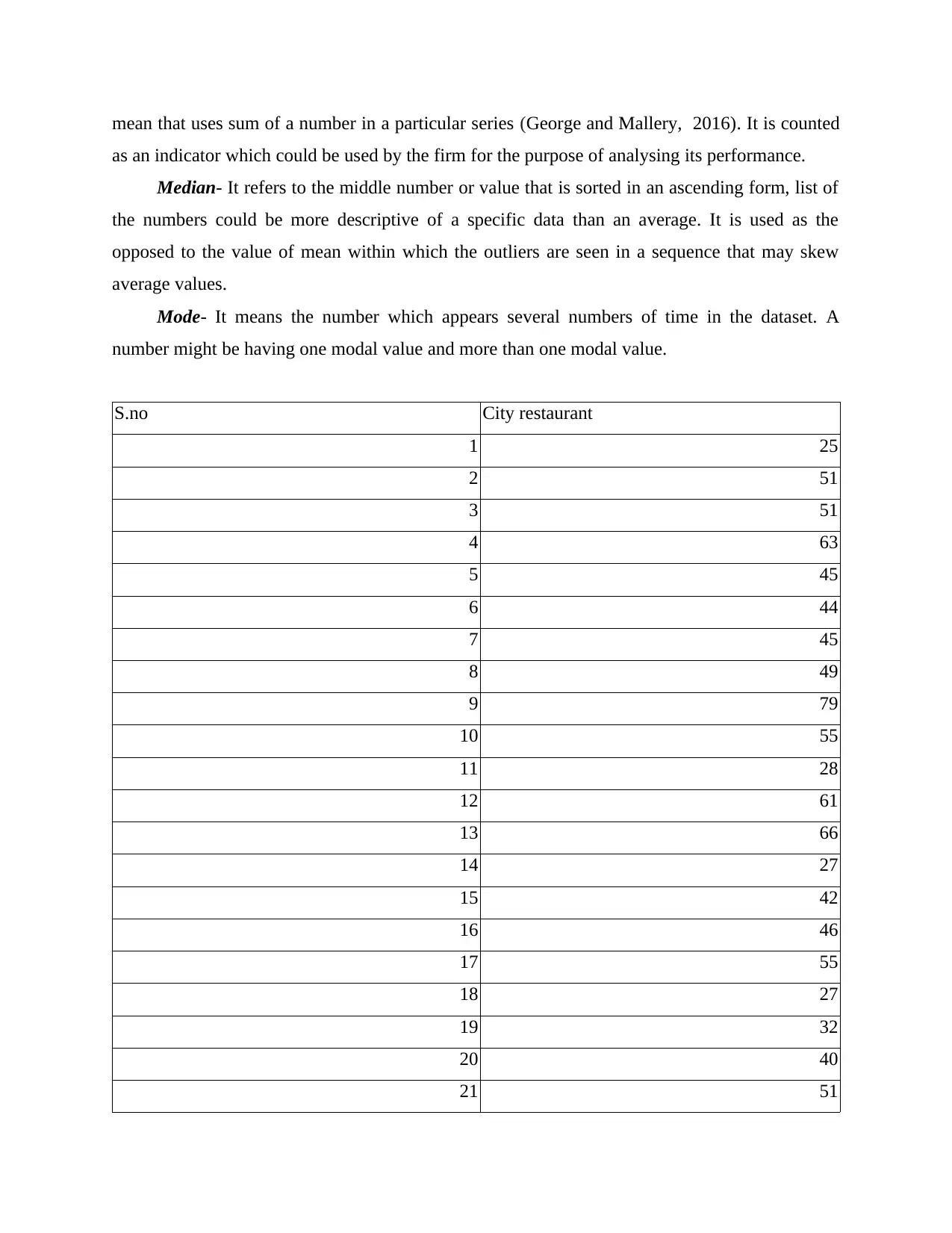
This report provides a comprehensive analysis of numerical data using various quantitative methods. It begins with an introduction to statistical tools and their application in data analysis. The report then delves into frequency distribution, presenting tables and interpretations for city and suburban restaurants. It proceeds to calculate the mean, median, and mode for both restaurant types. Further analysis includes the calculation of standard deviation for annual sales, the inter-quartile range for advertising expenses, and the coefficient of correlation. The report also conducts a regression analysis to examine the relationship between advertising expenditure and sales, interpreting the results and evaluating the coefficient of determination. Additionally, it explores probability calculations related to recruitment and training and discusses the applicability of the z-test. The report concludes with a summary of findings and references.

Applied Quantitative Methods

Table of Contents
INTRODUCTION...........................................................................................................................3
Question 1........................................................................................................................................3
c. On the basis of the raw data calculation of the mean, median and the mode..........................5
Question 2........................................................................................................................................9
a. Stating the difference between the sample and the population................................................9
b. Calculation of the standard deviation of an annual sales ......................................................10
c. Computing inter-quartile range relating to the annual advertising expenses ........................11
d. Computing coefficient of the correlation ..............................................................................12
Question 3......................................................................................................................................13
a. Explaining a selection of the dependent and an independent variable among the dataset of
annual sales and annual advertising expenses ..........................................................................13
b. Computing regression equation and interpreting the results .................................................14
c. Presenting an evaluation of coefficient determination and interpreting the finding
accordingly in order to analyse the dataset regarding the annual sales and the promotional
expenses.....................................................................................................................................16
Question 4......................................................................................................................................16
a. Calculating the probability ....................................................................................................17
b. ................................................................................................................................................17
c..................................................................................................................................................17
d. Explaining the relationship between recruitment and training .............................................18
Question 5......................................................................................................................................18
a..................................................................................................................................................18
b. ................................................................................................................................................19
CONCLUSION..............................................................................................................................19
REFERENCES................................................................................................................................1

INTRODUCTION
Quantitative methods details the different statistical and mathematical tools that are used
to analyse the numerical information that has been collected and then a synopsis is presented.
The statistical tools help in analysing the data that has been collected and then the results hence
drawn are interpreted accordingly (Liu and et.al., 2018). In the current report, the numerical data
has been assessed using different statistical concepts. Initially, the concept of frequency
distribution has been used and a histogram will be presented for the data related to the
restaurants. Then, the report will involve calculation of standard deviation and the correlation
coefficient will be calculated based on the data presented. The report will also present a
regression analysis and the coefficient of determination will be calculated for the advertising
expenditure that company incurred and the sales concurrent. In the next section, the report will
calculate probability of the cricket team by analysing the training and the associated recruitment.
Finally, the report will identify whether r z test can be applied on a non-normal distribution and
the situation of hedge fund manager will be analysed.
Question 1
Frequency distribution- It is the table that depicts a frequency of the several outcomes in
the sample. Each and every entry in a table reflects a frequency or the count of an occurrences of
the values in the particular or the specific group. The table below summarizes distribution of the
values within the sample. In the statistics, the table of the frequency distribution tells about the
number of an occurrences by way of organizing the raw data in an appropriate manner.
Count of City restaurant
City restaurant
Freq
uenc
y
25-34 8
35-44 12
45-54 13
55-64 9
65-74 3
75-84 2

85-94 3
Grand Total 50
Count of Suburban
restaurant
Suburban restaurant
Freq
uenc
y
27-36 10
37-46 21
47-56 13
57-66 2
67-76 2
77-86 1
87-96 1
Grand Total 50
Interpretation- The table presented above shows the frequency distribution of both types
of the restaurant that is City and the Suburban restaurant. As per the 50-sample taken of the city
restaurant the highest frequency resulted as 13 that lies between the class interval of 45-54 and
the lowest frequency as 2 that is the range of 75-84. Similarly, by reviewing the frequency
distribution of Suburban restaurant the highest and the lowest value of frequency resulted as 21
and 1 that lies in a range of 37-46 & 87-96.
Cumulative and relative frequency
Suburban
restaurant Total
Cumulative
frequency
Relative
frequency Mid-point
27-36 10 10 0.2 45
37-46 21 31 0.42 60
47-56 13 44 0.26 75
57-66 2 46 0.04 90
67-76 2 48 0.04 105
77-86 1 49 0.02 120

87-96 1 50 0.02 135
Grand
Total 50 100 1
City
restaurant Total
Cumulative
frequency Relative frequency
25-34 8 8 0.16 42
35-44 12 20 0.24 57
45-54 13 33 0.26 72
55-64 9 42 0.18 87
65-74 3 45 0.06 102
75-84 2 47 0.04 117
85-94 3 50 0.06 132
Grand
Total 50 100 1
c. On the basis of the raw data calculation of the mean, median and the mode
Mean- It refers to the mathematical average of the set of a two and more of the numbers.
The mean for given dataset could be computed in various ways with an inclusion of an arithmetic

mean that uses sum of a number in a particular series (George and Mallery, 2016). It is counted
as an indicator which could be used by the firm for the purpose of analysing its performance.
Median- It refers to the middle number or value that is sorted in an ascending form, list of
the numbers could be more descriptive of a specific data than an average. It is used as the
opposed to the value of mean within which the outliers are seen in a sequence that may skew
average values.
Mode- It means the number which appears several numbers of time in the dataset. A
number might be having one modal value and more than one modal value.
S.no City restaurant
1 25
2 51
3 51
4 63
5 45
6 44
7 45
8 49
9 79
10 55
11 28
12 61
13 66
14 27
15 42
16 46
17 55
18 27
19 32
20 40
21 51

22 28
23 62
24 86
25 55
26 80
27 49
28 36
29 39
30 30
31 53
32 36
33 52
34 55
35 29
36 60
37 42
38 42
39 41
40 51
41 61
42 74
43 67
44 43
45 51
46 40
47 43
48 53
49 90
50 90
Mean 50.4
Median 50

Mode 51
City restaurant
Mean 50.9183673
Median 51
Mode 51
Standard
Deviation 16.1230125
Range 63
Minimum 27
Maximum 90
Sum 2495
Count 49
Interpretation- From the above analysis it has been analysed that the mean value of the
city restaurant resulted as 50.97 which is depicted as the average value of the dataset. It is
represented as the centre of a particular data and is determined by dividing the sum of the
frequency with that of the total number of an observation. The median value which is referred as
the mid value of the statistical data and is computed by applying the formula that is (n+1)/2
through which an observation that contains the value of median could be evaluated (Signorell,
and et.al., 2016). With respect to the data of city restaurant, the median value is presented as 51.
Moreover, the modal value of the city restaurant data accounted as 51 which reflects as the
number that is repeated frequently in the data which in turn also means that probability of an
individual in visiting the restaurant is said as 51 times.
S.no. Suburban restaurant
1 33
2 31
3 46
4 50
5 56
6 49
7 46
8 38
9 46

10 34
11 41
12 40
13 37
14 47
15 36
16 46
17 46
18 54
19 39
20 39
21 45
22 28
23 30
24 52
25 30
26 52
27 42
28 46
29 39
30 31
31 55
32 32
33 49
34 55
35 40
36 60
37 42
38 27
39 41
40 48

41 61
42 70
43 74
44 43
45 51
46 40
47 43
48 53
49 80
50 89
Mean 46.04
Median 45.5
Mode 46
Suburban restaurant
Mean 46.3061224
Median 46
Mode 46
Standard
Deviation 12.8130859
Range 62
Minimum 27
Maximum 89
Sum 2269
Count 49
Interpretation- the above evaluation depicts that the mean value of the suburban restaurant
data ascertained as 46.3 which seems to be lower than the city restaurant. This reflects an
average value of the data which shows that averagely 46.3 times the customers prefer to go for a
suburban restaurant. It also shows that the meal cost at suburban restaurant highly differs from
the city restaurant. The median value resulted as 46 the which is very close to the mean value
and indicated as the middle value of the dataset (Opp, 2019). Further, the mode of the suburban
restaurant attained as 46 which considered as the value that is been highly repeated in the dataset.
Moreover, the standard deviation equates to 12.81 and the range which is seen as the difference
between smallest and the largest value resulted as 62.

Question 2
a. Stating the difference between the sample and the population
Population Sample
It is referred as the particular interest group
and under this the measurable quality is known
as the parameter.
It means as the subset or part of the population
and under this the measurable quality is been
called as statistic.
The population is considered as the compete
set of the data.
It represents the data regarding the part of the
population.
Under this, the reports are seen as the true
representation of an opinion.
Under this the reports are having an error
margin and the confidence interval.
It consist of all the members of the specific
group.
It is the part which represents an entire
population.
The data shown is been reflected as the sample because it presents the data in relation to
the annual sales and an advertising expenditure of a particular supermarket and not the data of an
entire population. It represents the dataset of the supermarket stating its annual sales and the
advertising expenses that has been incurred on an annual basis.
b. Calculation of the standard deviation of an annual sales
Product Annual sales(in 1000) (x) X^2
1 150 22500
2 150 22500
3 190 36100
4 130 16900
5 120 14400
6 110 12100
7 160 25600
8 180 32400
9 180 32400
10 150 22500

11 160 25600
12 140 19600
Total 1820 282600
Standard deviation= Square root of ∑x^2 / N – (∑x / n) ^ 2
= SQRT of (282600 / 12) – (1820 / 10) ^ 2
= SQRT of 23550 – 23002
= SQRT of 547.22
= 24.43
Interpretation- From the above assessment it has been identified that the standard
deviation of an annual sales of the supermarket evaluated as 24.43 which shows the dispersion
value from the mean. It is calculated by applying the formula and thereafter making the square
root of the value that is been attained from an equation or the formula. As the value of standard
deviation within the dataset is seen as large which clearly states that it is largely disperses from
the mean value or an average value and not depicted as close to the average or mean value.
c. Computing inter-quartile range relating to the annual advertising expenses
STEP 1 Arranging data in ascending order
Product Annual advertising expenditure
1 20
2 20
3 30
4 30
5 30
6 40
7 60
8 60
9 60
10 70
11 90