Statistical Data Collection and Interpretation Assessment Report

This report presents a comprehensive statistical analysis of employee data, encompassing data collection methods, descriptive statistics, and graphical analysis to understand the nature of the variables. The analysis includes correlation and regression techniques to examine relationships between variables like monthly salary and expense, with a strong positive linear relationship observed. Hypothesis tests, such as independent samples t-tests, one-way ANOVA, and chi-square tests, are employed to assess differences in means and independence between categorical variables. The findings reveal significant differences in TV hours between genders and salary/expense differences based on education levels, while other hypotheses are rejected. The study concludes with a detailed discussion of the results and their implications.

Statistical Data Collection and Interpretation
Assessment Item 3

Table of Contents
Abstract................................................................................................................................3
Introduction..........................................................................................................................3
Research Hypotheses............................................................................................................4
Data Collection.....................................................................................................................5
Descriptive Statistics............................................................................................................4
Graphical Analysis...............................................................................................................5
Correlation and Regression Analysis...................................................................................3
Independent Samples t-tests.................................................................................................3
One way ANOVA................................................................................................................4
Chi square test......................................................................................................................5
Results and Discussions.......................................................................................................4
Conclusions..........................................................................................................................5
References............................................................................................................................5
2 | P a g e

Assessment Item 3
Statistical Data Collection and Interpretation
Abstract
The correlation coefficient between the two variables monthly salary and monthly expense is
given as 0.957, which indicate a strong positive linear relationship. We conclude that there is a
statistically significant linear relationship exists between the two variables monthly salary and
monthly expense. No any statistically significant difference is observed between the average
monthly salary and expense for the female and male employees. A significant difference is
observed in the average number of TV hours for the female and male employees. No any
significant difference is observed in the average number of hours for exercise for male and
female employees. A significant difference is observed in the average monthly salary and
expense for the employees with different educations. Two categorical variables found
statistically independent from each other.
Introduction
Statistical data analysis plays an important role in the process of decision making in many
sectors. It is important to use proper statistical tools and techniques for data analysis. Here, we
have to analyse the data for the different variables regarding the employees. We have to draw the
conclusions for the variables such as gender, age, education, monthly salary, monthly expense,
etc. We have to use descriptive statistics, graphical analysis, correlation and regression,
hypotheses tests such as independent samples t tests and one factor ANOVA tests for checking
different claims regarding the variables. Let us see this statistical analysis in detail.
Research Hypotheses
For this study of statistical data collection and analysis, we consider the following research
hypotheses:
1. H0: There is no any statistically significant linear relationship exists between the two
variable monthly salary and monthly expense.
2. H0: There is no any significant difference exists between the average monthly salary for
the female and male employees.
3. H0: There is no any significant difference in average number of TV hours for female and
male employees.
3 | P a g e

4. H0: There is no any significant difference in the average number of hours for exercise for
male and female employees.
5. H0: There is no any significant difference in the average monthly salary for the
employees with different educations.
6. H0: There is no any statistically significant difference in the average monthly expense for
the employees with different education levels.
7. H0: There is no any statistically significant difference in the average number of TV hours
for the employees with different education levels.
8. H0: There is no any statistically significant difference in the average number of exercise
hours for the employees with different education levels.
9. H0: Two categorical variables gender and education levels are independent from each
other.
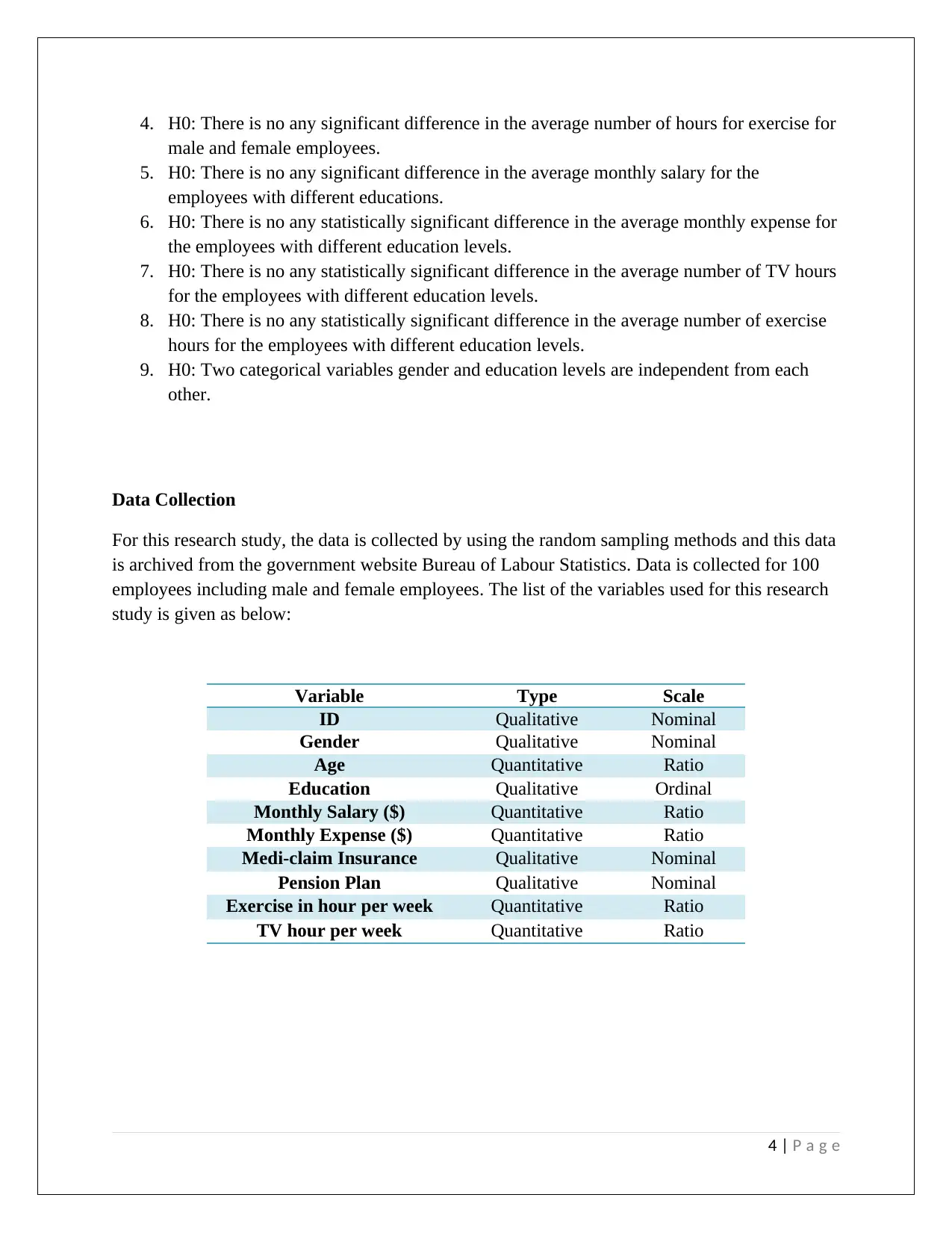
Data Collection
For this research study, the data is collected by using the random sampling methods and this data
is archived from the government website Bureau of Labour Statistics. Data is collected for 100
employees including male and female employees. The list of the variables used for this research
study is given as below:
Variable Type Scale
ID Qualitative Nominal
Gender Qualitative Nominal
Age Quantitative Ratio
Education Qualitative Ordinal
Monthly Salary ($) Quantitative Ratio
Monthly Expense ($) Quantitative Ratio
Medi-claim Insurance Qualitative Nominal
Pension Plan Qualitative Nominal
Exercise in hour per week Quantitative Ratio
TV hour per week Quantitative Ratio
4 | P a g e

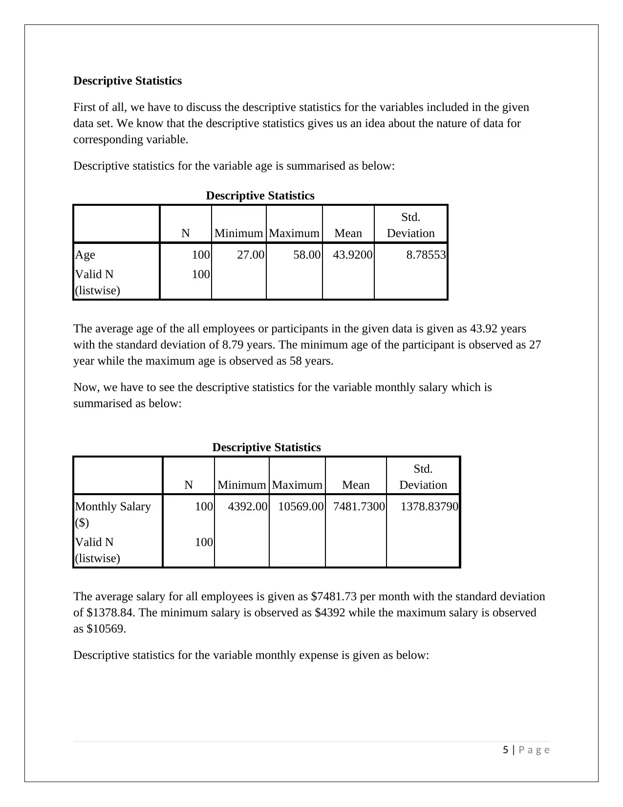
Descriptive Statistics
First of all, we have to discuss the descriptive statistics for the variables included in the given
data set. We know that the descriptive statistics gives us an idea about the nature of data for
corresponding variable.
Descriptive statistics for the variable age is summarised as below:
Descriptive Statistics
N Minimum Maximum Mean
Std.
Deviation
Age 100 27.00 58.00 43.9200 8.78553
Valid N
(listwise)
100
The average age of the all employees or participants in the given data is given as 43.92 years
with the standard deviation of 8.79 years. The minimum age of the participant is observed as 27
year while the maximum age is observed as 58 years.
Now, we have to see the descriptive statistics for the variable monthly salary which is
summarised as below:
Descriptive Statistics
N Minimum Maximum Mean
Std.
Deviation
Monthly Salary
($)
100 4392.00 10569.00 7481.7300 1378.83790
Valid N
(listwise)
100
The average salary for all employees is given as $7481.73 per month with the standard deviation
of $1378.84. The minimum salary is observed as $4392 while the maximum salary is observed
as $10569.
Descriptive statistics for the variable monthly expense is given as below:
5 | P a g e

Descriptive Statistics
N Minimum Maximum Mean
Std.
Deviation
Monthly Expense
($)
100 2081.00 9257.00 5643.8800 1478.30870
Valid N (listwise) 100
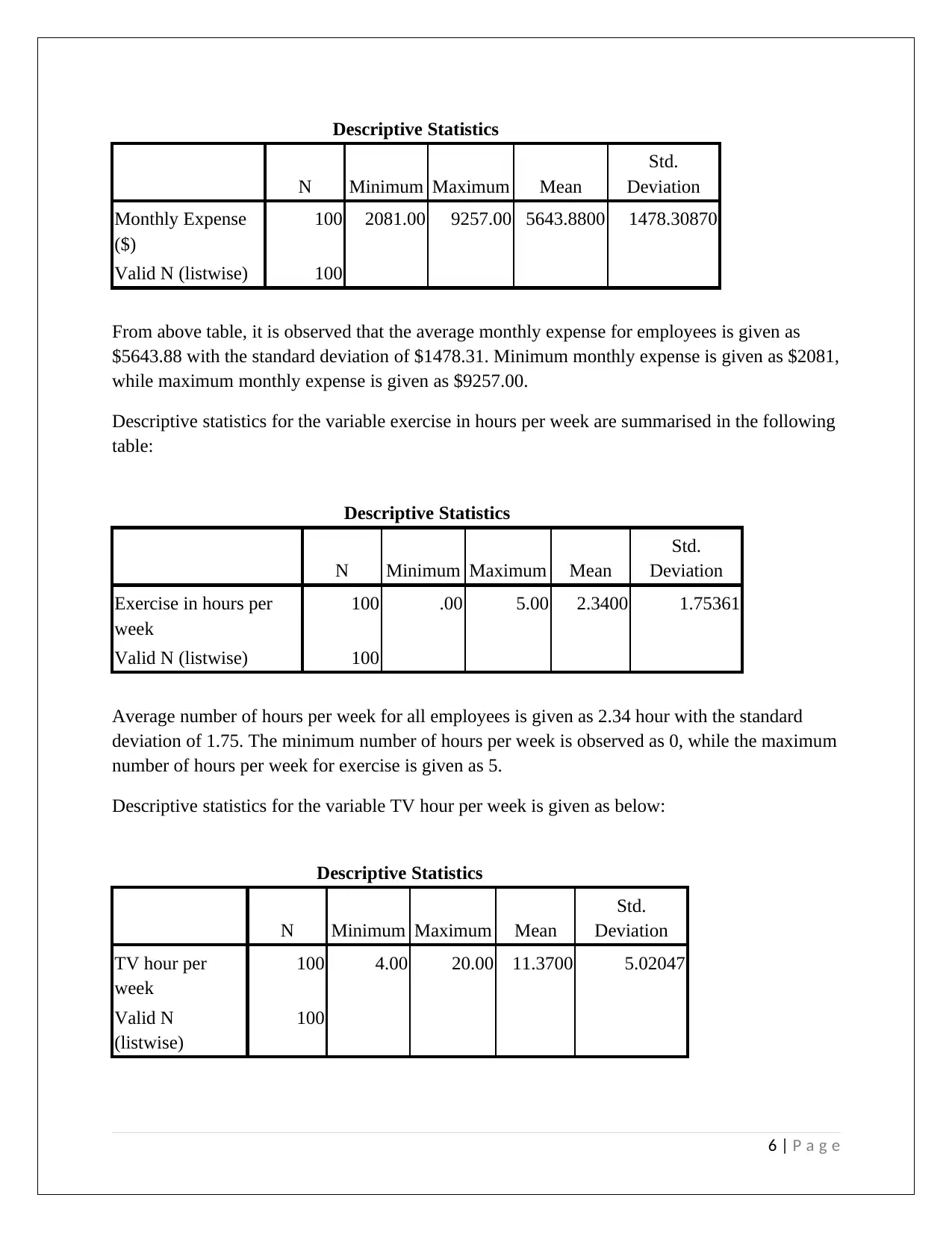
From above table, it is observed that the average monthly expense for employees is given as
$5643.88 with the standard deviation of $1478.31. Minimum monthly expense is given as $2081,
while maximum monthly expense is given as $9257.00.
Descriptive statistics for the variable exercise in hours per week are summarised in the following
table:
Descriptive Statistics
N Minimum Maximum Mean
Std.
Deviation
Exercise in hours per
week
100 .00 5.00 2.3400 1.75361
Valid N (listwise) 100
Average number of hours per week for all employees is given as 2.34 hour with the standard
deviation of 1.75. The minimum number of hours per week is observed as 0, while the maximum
number of hours per week for exercise is given as 5.
Descriptive statistics for the variable TV hour per week is given as below:
Descriptive Statistics
N Minimum Maximum Mean
Std.
Deviation
TV hour per
week
100 4.00 20.00 11.3700 5.02047
Valid N
(listwise)
100
6 | P a g e

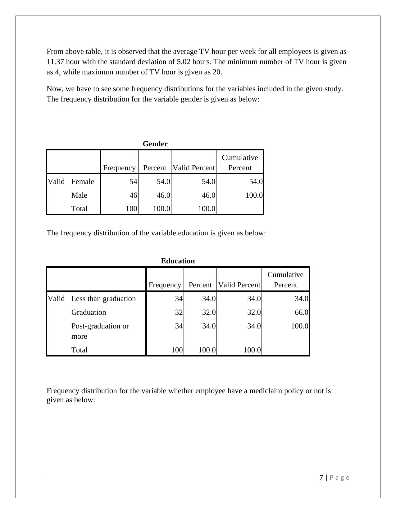
From above table, it is observed that the average TV hour per week for all employees is given as
11.37 hour with the standard deviation of 5.02 hours. The minimum number of TV hour is given
as 4, while maximum number of TV hour is given as 20.
Now, we have to see some frequency distributions for the variables included in the given study.
The frequency distribution for the variable gender is given as below:
Gender
Frequency Percent Valid Percent
Cumulative
Percent
Valid Female 54 54.0 54.0 54.0
Male 46 46.0 46.0 100.0
Total 100 100.0 100.0
The frequency distribution of the variable education is given as below:
Education
Frequency Percent Valid Percent
Cumulative
Percent
Valid Less than graduation 34 34.0 34.0 34.0
Graduation 32 32.0 32.0 66.0
Post-graduation or
more
34 34.0 34.0 100.0
Total 100 100.0 100.0
Frequency distribution for the variable whether employee have a mediclaim policy or not is
given as below:
7 | P a g e

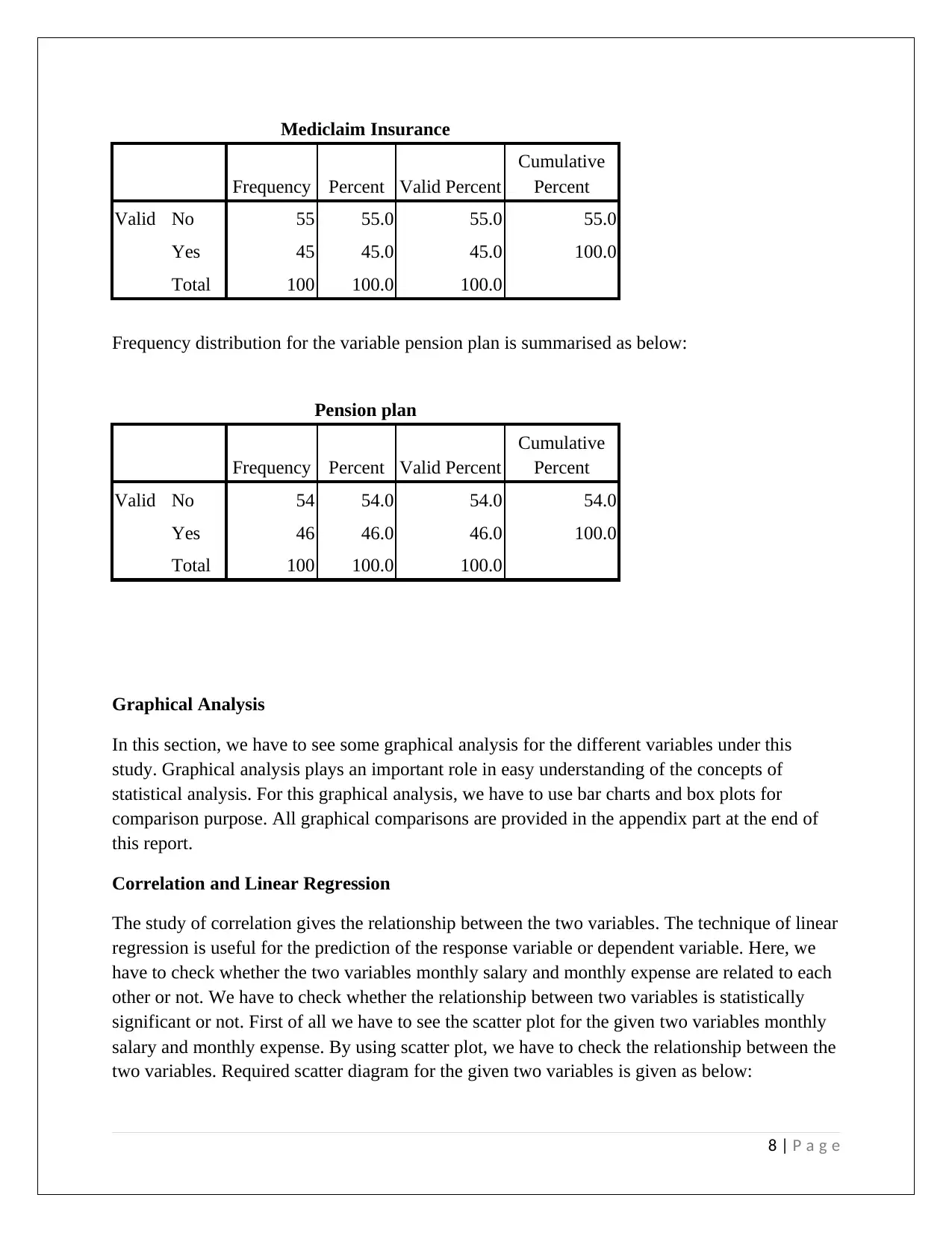
Mediclaim Insurance
Frequency Percent Valid Percent
Cumulative
Percent
Valid No 55 55.0 55.0 55.0
Yes 45 45.0 45.0 100.0
Total 100 100.0 100.0
Frequency distribution for the variable pension plan is summarised as below:
Pension plan
Frequency Percent Valid Percent
Cumulative
Percent
Valid No 54 54.0 54.0 54.0
Yes 46 46.0 46.0 100.0
Total 100 100.0 100.0
Graphical Analysis
In this section, we have to see some graphical analysis for the different variables under this
study. Graphical analysis plays an important role in easy understanding of the concepts of
statistical analysis. For this graphical analysis, we have to use bar charts and box plots for
comparison purpose. All graphical comparisons are provided in the appendix part at the end of
this report.
Correlation and Linear Regression
The study of correlation gives the relationship between the two variables. The technique of linear
regression is useful for the prediction of the response variable or dependent variable. Here, we
have to check whether the two variables monthly salary and monthly expense are related to each
other or not. We have to check whether the relationship between two variables is statistically
significant or not. First of all we have to see the scatter plot for the given two variables monthly
salary and monthly expense. By using scatter plot, we have to check the relationship between the
two variables. Required scatter diagram for the given two variables is given as below:
8 | P a g e

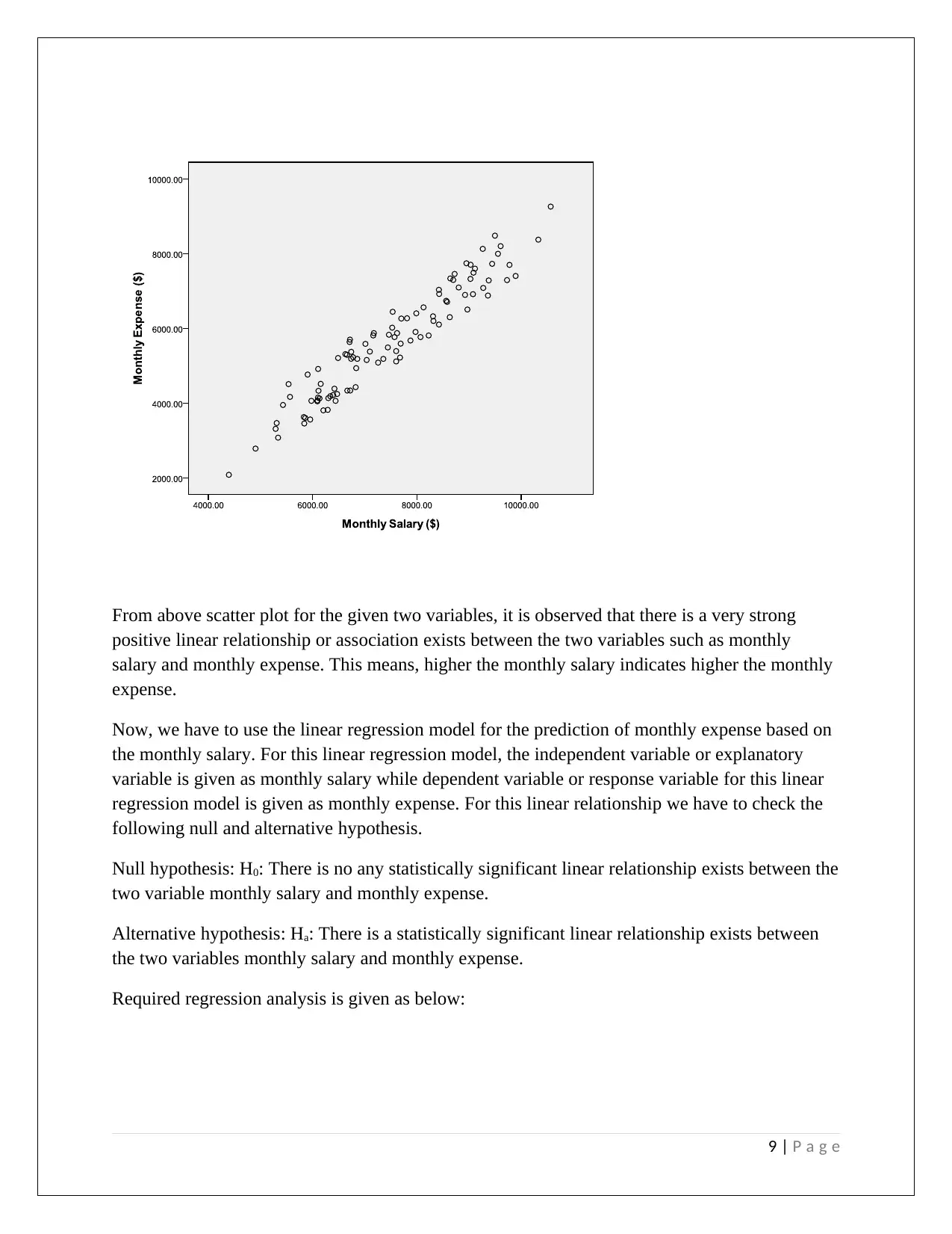
From above scatter plot for the given two variables, it is observed that there is a very strong
positive linear relationship or association exists between the two variables such as monthly
salary and monthly expense. This means, higher the monthly salary indicates higher the monthly
expense.
Now, we have to use the linear regression model for the prediction of monthly expense based on
the monthly salary. For this linear regression model, the independent variable or explanatory
variable is given as monthly salary while dependent variable or response variable for this linear
regression model is given as monthly expense. For this linear relationship we have to check the
following null and alternative hypothesis.
Null hypothesis: H0: There is no any statistically significant linear relationship exists between the
two variable monthly salary and monthly expense.
Alternative hypothesis: Ha: There is a statistically significant linear relationship exists between
the two variables monthly salary and monthly expense.
Required regression analysis is given as below:
9 | P a g e

Variables Entered/Removedb
Model
Variables
Entered
Variables
Removed Method
1 Monthly
Salary ($)a
. Enter
a. All requested variables entered.
b. Dependent Variable: Monthly Expense ($)
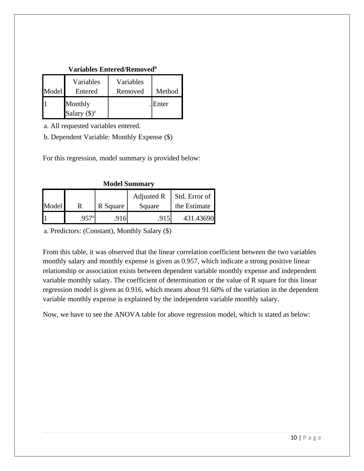
For this regression, model summary is provided below:
Model Summary
Model R R Square
Adjusted R
Square
Std. Error of
the Estimate
1 .957a .916 .915 431.43690
a. Predictors: (Constant), Monthly Salary ($)
From this table, it was observed that the linear correlation coefficient between the two variables
monthly salary and monthly expense is given as 0.957, which indicate a strong positive linear
relationship or association exists between dependent variable monthly expense and independent
variable monthly salary. The coefficient of determination or the value of R square for this linear
regression model is given as 0.916, which means about 91.60% of the variation in the dependent
variable monthly expense is explained by the independent variable monthly salary.
Now, we have to see the ANOVA table for above regression model, which is stated as below:
10 | P a g e

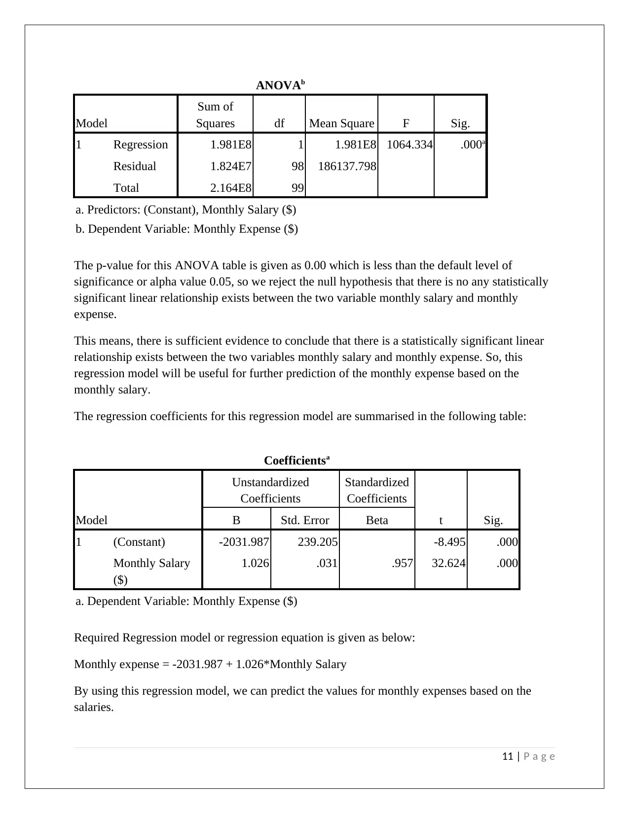
ANOVAb
Model
Sum of
Squares df Mean Square F Sig.
1 Regression 1.981E8 1 1.981E8 1064.334 .000a
Residual 1.824E7 98 186137.798
Total 2.164E8 99
a. Predictors: (Constant), Monthly Salary ($)
b. Dependent Variable: Monthly Expense ($)
The p-value for this ANOVA table is given as 0.00 which is less than the default level of
significance or alpha value 0.05, so we reject the null hypothesis that there is no any statistically
significant linear relationship exists between the two variable monthly salary and monthly
expense.
This means, there is sufficient evidence to conclude that there is a statistically significant linear
relationship exists between the two variables monthly salary and monthly expense. So, this
regression model will be useful for further prediction of the monthly expense based on the
monthly salary.
The regression coefficients for this regression model are summarised in the following table:
Coefficientsa
Model
Unstandardized
Coefficients
Standardized
Coefficients
t Sig.B Std. Error Beta
1 (Constant) -2031.987 239.205 -8.495 .000
Monthly Salary
($)
1.026 .031 .957 32.624 .000
a. Dependent Variable: Monthly Expense ($)
Required Regression model or regression equation is given as below:
Monthly expense = -2031.987 + 1.026*Monthly Salary
By using this regression model, we can predict the values for monthly expenses based on the
salaries.
11 | P a g e

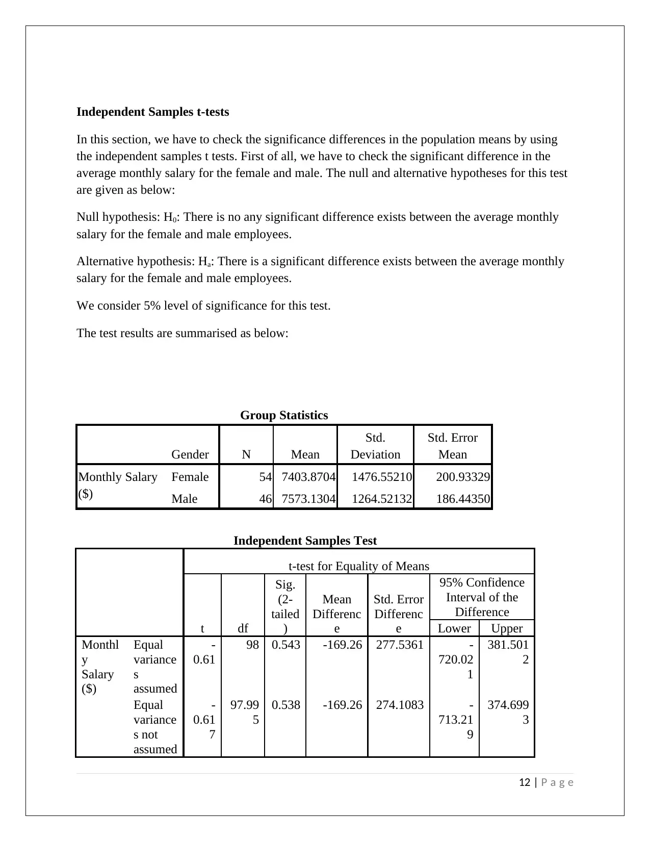
Independent Samples t-tests
In this section, we have to check the significance differences in the population means by using
the independent samples t tests. First of all, we have to check the significant difference in the
average monthly salary for the female and male. The null and alternative hypotheses for this test
are given as below:
Null hypothesis: H0: There is no any significant difference exists between the average monthly
salary for the female and male employees.
Alternative hypothesis: Ha: There is a significant difference exists between the average monthly
salary for the female and male employees.
We consider 5% level of significance for this test.
The test results are summarised as below:
Group Statistics
Gender N Mean
Std.
Deviation
Std. Error
Mean
Monthly Salary
($)
Female 54 7403.8704 1476.55210 200.93329
Male 46 7573.1304 1264.52132 186.44350
Independent Samples Test
t-test for Equality of Means
t df
Sig.
(2-
tailed
)
Mean
Differenc
e
Std. Error
Differenc
e
95% Confidence
Interval of the
Difference
Lower Upper
Monthl
y
Salary
($)
Equal
variance
s
assumed
-
0.61
98 0.543 -169.26 277.5361 -
720.02
1
381.501
2
Equal
variance
s not
assumed
-
0.61
7
97.99
5
0.538 -169.26 274.1083 -
713.21
9
374.699
3
12 | P a g e