Statistical Methods in Engineering Homework - University, 2018

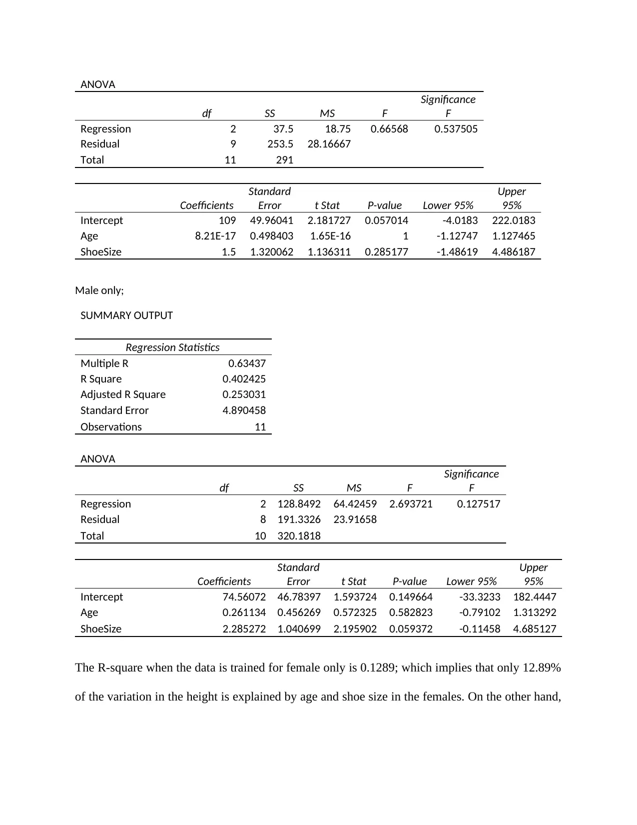
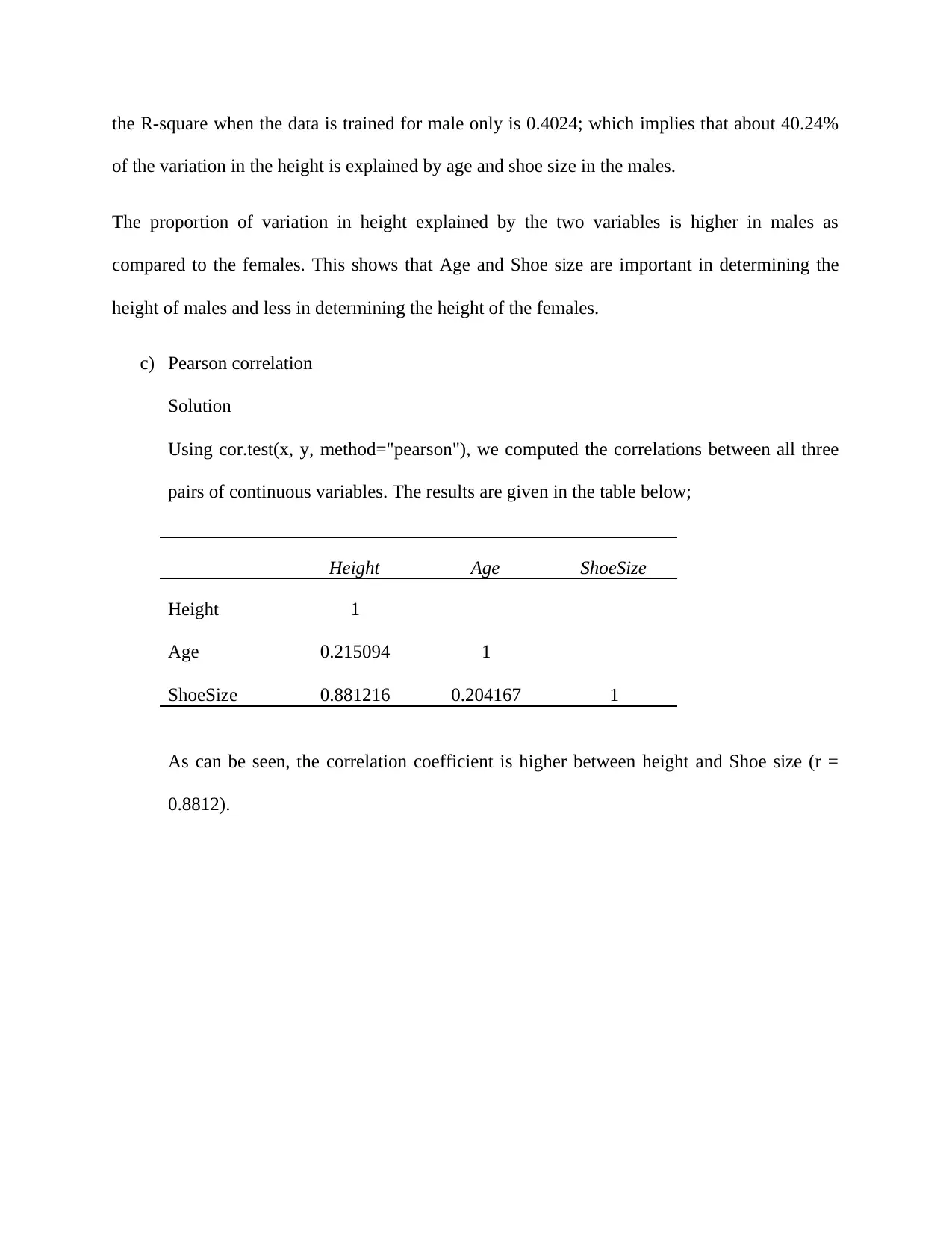
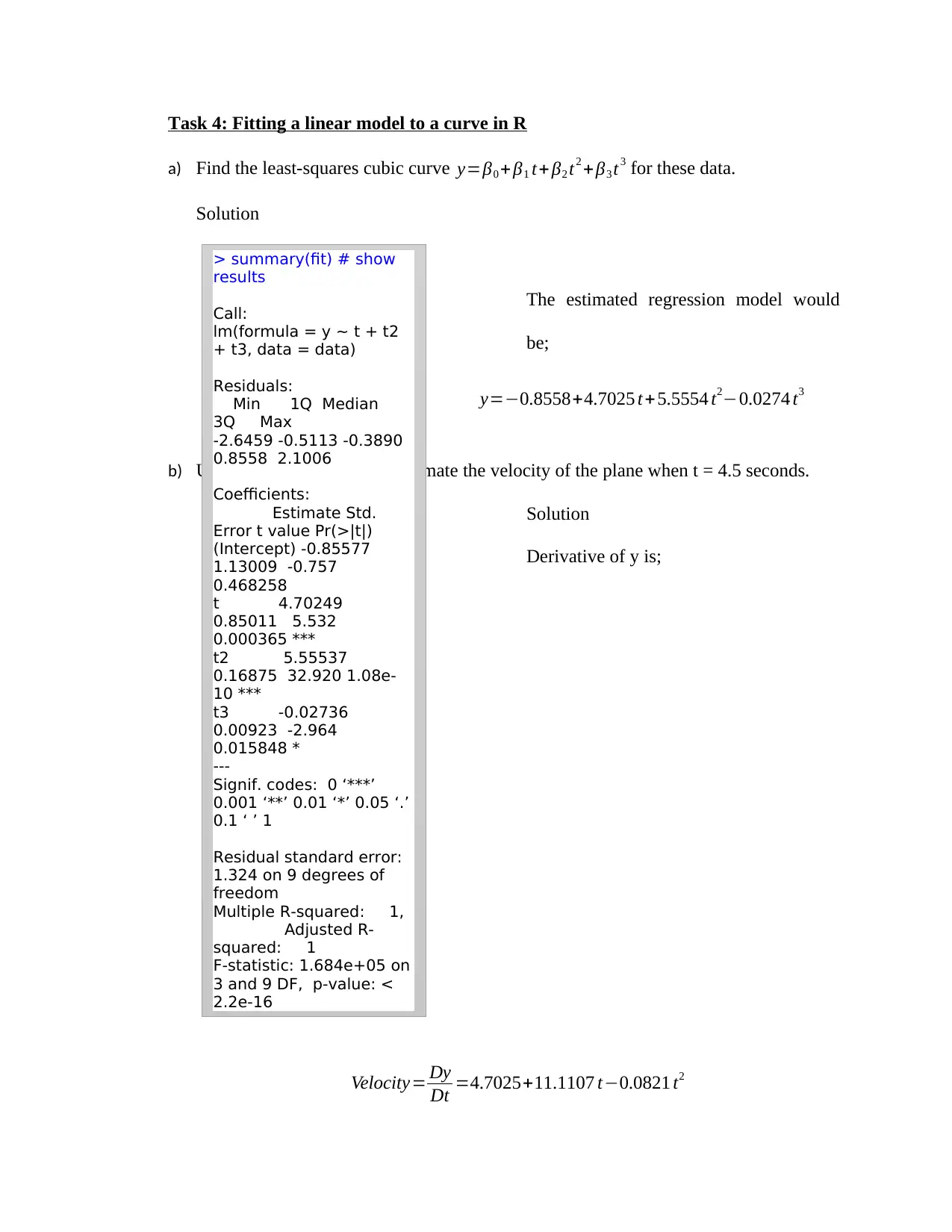
This document presents a comprehensive solution to a statistical methods in engineering assignment. It begins with an explanation of the Gram-Schmidt process for orthogonalization. The assignment then delves into linear models, including finding the equation of a least-squares line and analyzing data using Excel. The Excel portion includes regression statistics, ANOVA tables, and the development of estimated linear regression models, with separate analyses for male and female data. The document also explores Pearson correlation. Finally, the assignment addresses fitting a linear model to a curve using R, including interpreting regression output and estimating the velocity of a plane using derivatives. The solution provides detailed steps and interpretations for each task, offering a complete understanding of the statistical concepts involved.

Statistical Methods in Engineering
Student Name:
University
15th January 2018

Task 1: Orthogonalization
According to the Gram-Schmidt Process. If we let V to be an inner product space
and {v1 , v2 , ... , vn } to be a set of linearly independent vectors that are in V. Then there exists an
orthonormal set of vectors {e1 , e2 , ..., en } of V such that span ( v1 , v2 ,... , v j ) =span(e1 ,e2 ,... , e j ) for
each j=1 ,2 , ..., n.
The proof is done by induction.
Suppose j=1; we can then let e1=v1 ∥v1 ∥. But ∥ v1 ∥ ≠ 0 since v1 ≠ 0 bearing in mind that a set of
linearly independent vectors has no zero vector. From this it is clear that span(v1)=span( e1 )
based on the fact that v1 and e1 differ only by ∥ v1 ∥ as such they are scalar multiples of each
other. Again, ∥e1 ∥=∥ v1 ∥ ∥v1 ∥=1.
Next considering the case when j>1, and assuming a set of orthonormal vectors of j−1
, {e1 , e2 , ..., e j−1 } such that span( v1 , v2 , ..., v j−1)=span (e1 , e2 , ... , e j−1). Now since {v1 , v2 , ... , vn }
is a linearly independent set of vectors, we have that v j ∉ span (v1 , v2 ,... , v j−1). Thus we define
the vector ej as:
e j = v j−¿ v j , e1> e1−¿ v j , e2> e2−...−¿ v j , e j−1 >e j−1
∥ v j−¿ v j , e1> e1−¿ v j , e2> e2−...−¿ v j , e j−1 >e j−1 ∥
Clearly∥ e j ∥=1. Next is to show that e j is orthonormal to e1 ,e2 ,... , e j−1. Given any integer k
such that 1 ≤ k< j, we consider the inner product of e jwith ek. Le
t N=∥ v j −¿ v j , e1>e1 −¿ v j , e2> e2 −...−¿ v j , e j−1> e j−1 ∥. Then we have that:
⟨ e j , ek ⟩ = ⟨ v j−¿ v j , e1 >e1−¿ v j , e2 >e2−...−¿ v j , e j−1 >e j−1
N , ek ⟩
¿ 1
N ⟨ v j−¿ v j , e1 >e1−¿ v j , e2 >e2−...−¿ v j , e j−1>e j−1 , ek ⟩
¿ 1
N ( ⟨ v j , ek ⟩ − ⟨ v j , ek ⟩ )=0
Now it is clear that the set of vectors {e1 , e2 , ..., e j } is orthonormal. It is therefore evident
that
span ( v1 , v2 ,... , v j ) =span(e1 ,e2 ,... , e j )

Task 2: Linear models by hand
a) observation vector ⃗ y and evidence matrix X
Solution
Observation vector is;⃗
y=
[0
1
2
4 ]Evidence matrix is;
X =
[ 1 −1
1 0
1
1
1
2 ]b) We sought to find the equation y=β0 +β1 x of the least-squares line that best fits the
given data points.
Solution
^β= [ β0
β1 ] = ( X ' X ) −1
X' y=
([ 1 1 1 1
−1 0 1 2 ] [ 1 −1
1 0
1
1
1
2 ] )
−1
[ 1 1 1 1
−1 0 1 2 ] [ 0
1
2
4 ] = [−0.8000
0.7429 ]
Thus the equation is;
y=−0.8000+0.7429 x

Task 3: Linear models on the computer
Using Excel software, we obtain the following results;
SUMMARY OUTPUT
Regression Statistics
Multiple R 0.881948
R Square 0.777832
Adjusted R Square 0.755616
Standard Error 4.855596
Observations 23
ANOVA
df SS MS F
Significance
F
Regression 2 1650.899 825.4493 35.01107 2.93E-07
Residual 20 471.5362 23.57681
Total 22 2122.435
Coefficient
s
Standard
Error t Stat P-value Lower 95%
Upper
95%
Intercept 67.34771 13.66809 4.927369 8.12E-05 38.83658 95.85883
Age 0.109281 0.32052 0.34095 0.736697 -0.55931 0.777874
ShoeSize 2.525974 0.311263 8.115248 9.34E-08 1.876691 3.175257
a) The estimated linear regression model is;
Solution
Height =67.3477+0.1093 ( Age ) +2.5260 ¿
b) Training the data on only females and only males;
Solution
Female only:
SUMMARY OUTPUT
Regression Statistics
Multiple R 0.358979
R Square 0.128866
Adjusted R Square -0.06472
Standard Error 5.307228
Observations 12

ANOVA
df SS MS F
Significance
F
Regression 2 37.5 18.75 0.66568 0.537505
Residual 9 253.5 28.16667
Total 11 291
Coefficients
Standard
Error t Stat P-value Lower 95%
Upper
95%
Intercept 109 49.96041 2.181727 0.057014 -4.0183 222.0183
Age 8.21E-17 0.498403 1.65E-16 1 -1.12747 1.127465
ShoeSize 1.5 1.320062 1.136311 0.285177 -1.48619 4.486187
Male only;
SUMMARY OUTPUT
Regression Statistics
Multiple R 0.63437
R Square 0.402425
Adjusted R Square 0.253031
Standard Error 4.890458
Observations 11
ANOVA
df SS MS F
Significance
F
Regression 2 128.8492 64.42459 2.693721 0.127517
Residual 8 191.3326 23.91658
Total 10 320.1818
Coefficients
Standard
Error t Stat P-value Lower 95%
Upper
95%
Intercept 74.56072 46.78397 1.593724 0.149664 -33.3233 182.4447
Age 0.261134 0.456269 0.572325 0.582823 -0.79102 1.313292
ShoeSize 2.285272 1.040699 2.195902 0.059372 -0.11458 4.685127
The R-square when the data is trained for female only is 0.1289; which implies that only 12.89%
of the variation in the height is explained by age and shoe size in the females. On the other hand,

the R-square when the data is trained for male only is 0.4024; which implies that about 40.24%
of the variation in the height is explained by age and shoe size in the males.
The proportion of variation in height explained by the two variables is higher in males as
compared to the females. This shows that Age and Shoe size are important in determining the
height of males and less in determining the height of the females.
c) Pearson correlation
Solution
Using cor.test(x, y, method="pearson"), we computed the correlations between all three
pairs of continuous variables. The results are given in the table below;
Height Age ShoeSize
Height 1
Age 0.215094 1
ShoeSize 0.881216 0.204167 1
As can be seen, the correlation coefficient is higher between height and Shoe size (r =
0.8812).

Task 4: Fitting a linear model to a curve in R
a) Find the least-squares cubic curve y=β0 + β1 t+ β2 t2 +β3 t3 for these data.
Solution
The estimated regression model would
be;
y=−0.8558+4.7025 t+5.5554 t2−0.0274 t3
b) Using results in part (a) to estimate the velocity of the plane when t = 4.5 seconds.
Solution
Derivative of y is;
Velocity= Dy
Dt =4.7025+11.1107 t−0.0821 t2
> summary(fit) # show
results
Call:
lm(formula = y ~ t + t2
+ t3, data = data)
Residuals:
Min 1Q Median
3Q Max
-2.6459 -0.5113 -0.3890
0.8558 2.1006
Coefficients:
Estimate Std.
Error t value Pr(>|t|)
(Intercept) -0.85577
1.13009 -0.757
0.468258
t 4.70249
0.85011 5.532
0.000365 ***
t2 5.55537
0.16875 32.920 1.08e-
10 ***
t3 -0.02736
0.00923 -2.964
0.015848 *
---
Signif. codes: 0 ‘***’
0.001 ‘**’ 0.01 ‘*’ 0.05 ‘.’
0.1 ‘ ’ 1
Residual standard error:
1.324 on 9 degrees of
freedom
Multiple R-squared: 1,
Adjusted R-
squared: 1
F-statistic: 1.684e+05 on
3 and 9 DF, p-value: <
2.2e-16

Velocity=4.7025+11.1107∗4.5−0.0821 ¿ ( 4.5 ) 2 53.03813 feet / sec