Statistical Analysis of House Prices: Regression Project Report

This project report focuses on building and analyzing multiple linear regression models to predict house prices. The study utilizes factors such as lot size, number of bedrooms and bathrooms, the presence of a basement, and air conditioning to create both population and sample regression models. The analysis includes detailed interpretation of coefficients, assessment of statistical significance, and tests for outliers, heteroscedasticity, and multicollinearity. The findings reveal the significance of the models and identify the impact of each independent variable on house prices, along with the presence of multicollinearity between some variables. The report concludes with recommendations for model refinement and a discussion of the variables' predictive power.

Running head: Business analysis project 1
Panama Canal Expansion Project
Student name:
Course code:
Tutor:
1

Business analysis project 2
Table of Contents
1.0 Introduction................................................................................................................................4
2.0 Data analysis and results............................................................................................................4
2.1 Population regression model..................................................................................................4
2.2 Sample regression model.......................................................................................................5
2.3 Sample regression equation...................................................................................................5
2.4 Statistical significance of the regression model.....................................................................6
2.5 Interpretation of the coefficients of X1 to X5.........................................................................6
2.5.1 Population regression model...........................................................................................6
2.5.2 Sample regression model.................................................................................................6
2.6 Plots to check existence of outliers........................................................................................7
2.6.1 Lot size residual plot.......................................................................................................7
2.6.2 Bedroom residual plot.....................................................................................................7
2.6.3 Bathroom residual plot....................................................................................................8
2.6.4 Basement residual plot....................................................................................................8
2.6.5 Air condition residual plot...............................................................................................8
2.7 Heteroscedasticity test............................................................................................................9
2.7.1 Relationship between residual and lot size.........................................................................9
2.7.2 Relationship between residual and number of bedrooms...................................................9
2.7.3 Relationship between residual and number of bathrooms.............................................10
2.7.4 Relationship between residual and number of basement..............................................10
2.7.5 Relationship between residual and number of air condition.........................................11
2.8 Test for multicollinearity.....................................................................................................11
3.0 Conclusion...............................................................................................................................12
References.....................................................................................................................................13
Appendices....................................................................................................................................14

Business analysis project 3
Executive summary
The objective of this research Panama Canal expansion project report was to build a
model that would be used to predict the house prices using lot size, number of bedrooms, and
number of bathrooms, basement and presence of air conditioners. Multiple linear regression was
employed to come up with the model. The research study found and made several conclusions.
The models generated were very significant and could be used to predict the house prices. The
study also found out that there was a case of multicollinearity between number of bathrooms and
number of bedrooms. This could compromise the robustness of the model and therefore
recommended the removal of one of them when generating the model. It was also concluded that
all the independent variables were significant predictors of house prices except the basement.

Business analysis project 4
1.0 Introduction
In determining house prices, several variables come into play. Some of the variables
include lot size, number of bedrooms, and number of bathrooms, basement and presence of air
conditioners in the house (Abelson and Chung, 2015, pp. 265-280) and (Dongsheng and Zhong,
2010, pp. 3-7) The objective of this research report was to build a model that would be used to
predict the house prices using the mentioned variables. The results of the analysis are shown in
the next sections.
2.0 Data analysis and results
2.1 Population regression model
Result
SUMMARY
OUTPUT
Regression Statistics
Multiple R 0.756274
R Square 0.57195
Adjusted R
Square 0.567987
Standard Error 17551.05
Observations 546
ANOVA
df SS MS F
Significance
F
Regression 5
2.22262E+1
1
4445231035
9
144.307
3 4.65196E-97
Residual 540
1.66341E+1
1
308039322.
3
Total 545
3.88603E+1
1
Coefficient
s Std error t Stat P-value Lower 95%
Upper
95%
Intercept 50.26778 3475.93824
0.01446164
4 0.98846 -6777.74981 6878.28
lot size 4.736354 0.36115517
13.1144579
5
2.63E-
34
4.02691314
8 5.44579
#bedroom 4660.117 1109.44999 4.20038507 3.12E- 2480.75049 6839.48

Business analysis project 5
9 05 3
#bath 17594.49 1645.95745
10.6895162
1
2.53E-
24
14361.2247
3 20827.7
basement 6081.047 1587.20027
3.83130398
8 0.00014
2963.20325
2 9198.89
air condition 16130.42 1680.55406
9.59827716
7
3.01E-
20
12829.1991
3 19431.6
Table 2
The population regression model is as below;
House price=4.74 ¿
2.2 Sample regression model
SUMMARY
OUTPUT
Regression Statistics
Multiple R 0.78878434
R Square 0.622180734
Adjusted R Square 0.607649224
Standard Error 18101.17882
Observations 136
ANOVA
df SS MS F
Significance
F
Regression 5
7.01E+1
0 1.4E+10 42.8159 6.73683E-26
Residual 130
4.26E+1
0 3.28E+8
Total 135
1.13E+1
1
Coefficients Std error t Stat P-value Lower 95% Upper 95%
Intercept 4092.457496 7694.63 0.53185 0.59573 -11130.4491 19315.364
lot size 3.640791429 0.67461 5.39687 3.11E-7 2.30615296 4.9754298
#bedroom 5509.57759 2681.43 2.05471 0.04191 204.673455 10814.481
#bath 20402.65302 3207.07 6.36175 3.13E-9 14057.8305 26747.475
basement 4805.748585 3216.02 1.49431 0.13751 -1556.76554 11168.262
air cond 19103.00794 3247.91 5.88162 3.24E-8 12677.4040 25528.611
Table 2
The sample regression model is as below;

Business analysis project 6
House price=3.64 ¿
2.3 Sample regression equation
The sample regression model is as below;
House price=3.64 ¿
2.4 Statistical significance of the regression model
Both the regression models have (F = 0.00). This means that the models are significant since
there is 0.00% chance that the models just occurred by mere chance.
2.5 Interpretation of the coefficients of X1 to X5
2.5.1 Population regression model
House price=4.74 ¿
From the regression model above, it can be said that a one unit change in lot size causes
4.74 units increase in house price. A one unit change in the number of bedrooms causes 4660.12
units increase in house price. When it comes to the bathrooms, one unit change in the number of
bathrooms causes 17594.49 units increase in house price. To add on, a unit change in the number
of basement causes 6081.05 units increase in house price. Lastly, a unit change in the number of
air conditioners causes 16130.42 units increase in house price.
All the independent variables have p-values less than 0.05 which is the level of
significance. This means that all the independent variables in this model are significant (Haurin
and Gill, 2012, pp. 136-150)
2.5.2 Sample regression model
House price=3.64 ¿
From the regression model above, it can be said that a one unit change in lot size causes
3.64 units increase in house price. A one unit change in the number of bedrooms causes 5509.58
units increase in house price. When it comes to the bathrooms, one unit change in the number of
bathrooms causes 20402.65 units increase in house price. To add on, a unit change in the number
of basement causes 4805.75 units increase in house price. Lastly, a unit change in the number of
air conditioners causes 19103 units increase in house price.

Business analysis project 7
All the independent variables have p-values less than 0.05 which is the level of
significance except basement. This means that all the independent variables except basement are
significant (Hua, 2018, pp. 11-13)
2.6 Plots to check existence of outliers
2.6.1 Lot size residual plot
0
2000
4000
6000
8000
10000
12000
14000
16000
18000
-100000
-50000
0
50000
100000
lot size Residual Plot
lot size
Residuals
Figure 1
There is no presence of outliers as can be observed from the plot.
2.6.2 Bedroom residual plot
0 1 2 3 4 5 6 7
-100000
-50000
0
50000
100000
#bedroom Residual Plot
#bedroom
Residuals
Figure 2
There is no presence of outliers as can be observed from the plot

Business analysis project 8
2.6.3 Bathroom residual plot
0.5 1 1.5 2 2.5 3 3.5 4 4.5
-100000
-50000
0
50000
100000
#bath Residual Plot
#bath
Residuals
Figure 3
There is no presence of outliers as can be observed from the plot
2.6.4 Basement residual plot
0 0.2 0.4 0.6 0.8 1 1.2
-100000
-50000
0
50000
100000
basement Residual Plot
basement
Residuals
Figure 4
As can be observed from the plot, there is one outlier value (84,846.11).

Business analysis project 9
2.6.5 Air condition residual plot
0 0.2 0.4 0.6 0.8 1 1.2
-100000
-50000
0
50000
100000
air cond Residual Plot
air cond
Residuals
Figure 5
There is no presence of outliers as can be observed from the plot
2.7 Heteroscedasticity test
2.7.1 Relationship between residual and lot size
-60000 -40000 -20000 0 20000 40000 60000 80000 100000
0
2000
4000
6000
8000
10000
12000
14000
16000
18000
f(x) = − 4.30132852787387E-17 x + 6545.07352941176
R² = 3.33066907387547E-16
lot size vs residual
Residual
Lot size
Figure 6
As can be observed from figure 6 above, the line of best fit is horizontal. To add on the
value of r-squared is 0.00. The horizontal line means there is no relationship between the lot size
and residuals (Karantonis and Ge, 2007, pp. 493-509). R-squared value means that the residual is
not responsible for any variation that occurs in lot size.

Business analysis project
10
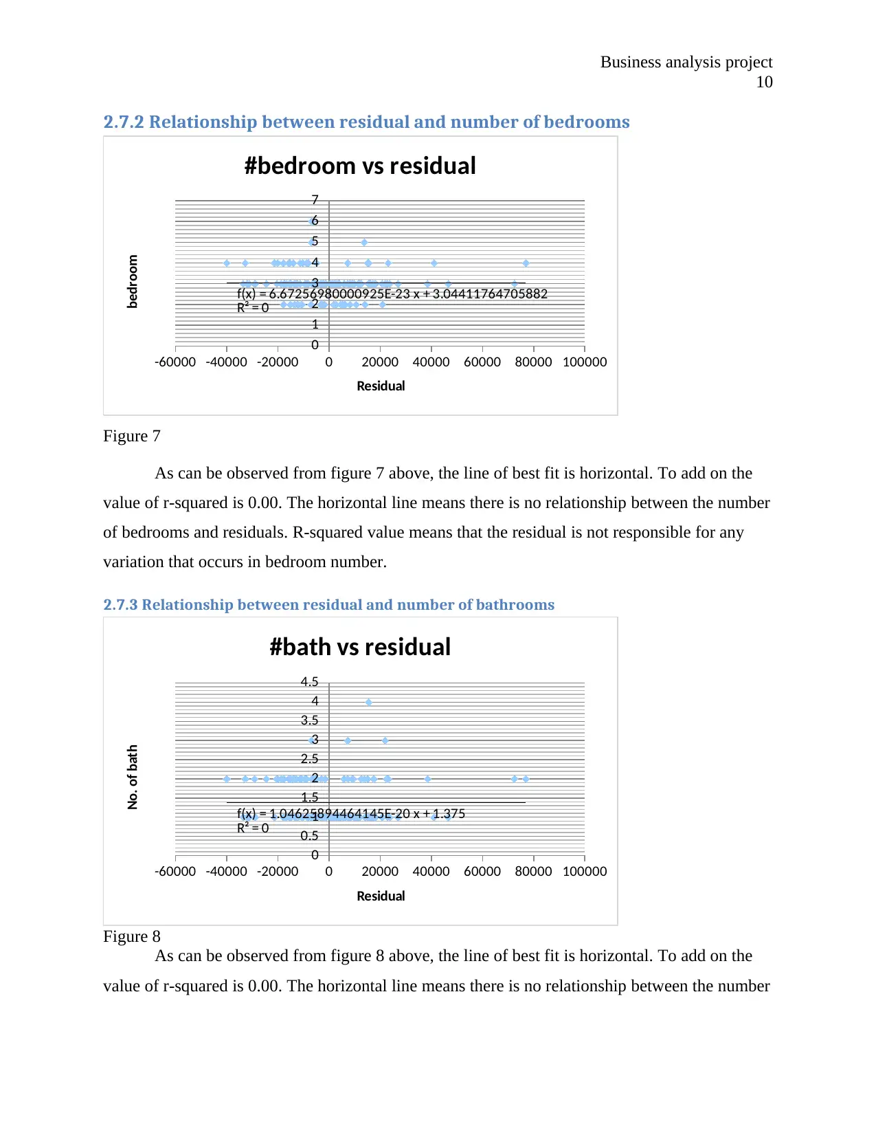
2.7.2 Relationship between residual and number of bedrooms
-60000 -40000 -20000 0 20000 40000 60000 80000 100000
0
1
2
3
4
5
6
7
f(x) = 6.67256980000925E-23 x + 3.04411764705882
R² = 0
#bedroom vs residual
Residual
bedroom
Figure 7
As can be observed from figure 7 above, the line of best fit is horizontal. To add on the
value of r-squared is 0.00. The horizontal line means there is no relationship between the number
of bedrooms and residuals. R-squared value means that the residual is not responsible for any
variation that occurs in bedroom number.
2.7.3 Relationship between residual and number of bathrooms
-60000 -40000 -20000 0 20000 40000 60000 80000 100000
0
0.5
1
1.5
2
2.5
3
3.5
4
4.5
f(x) = 1.04625894464145E-20 x + 1.375
R² = 0
#bath vs residual
Residual
No. of bath
Figure 8
As can be observed from figure 8 above, the line of best fit is horizontal. To add on the
value of r-squared is 0.00. The horizontal line means there is no relationship between the number

Business analysis project
11
of bathrooms and residuals. R-squared value means that the residual is not responsible for any
variation that occurs in bathroom number.
2.7.4 Relationship between residual and number of basement
-60000 -40000 -20000 0 20000 40000 60000 80000 100000
0
0.2
0.4
0.6
0.8
1
1.2
f(x) = 6.10673588096847E-21 x + 0.397058823529412
R² = 2.22044604925031E-16
Basement vs residual
Residual
Basement
Figure 9
As can be observed from figure 9 above, the line of best fit is horizontal. To add on the
value of r-squared is 0.00. The horizontal line means there is no relationship between basement
and residuals. R-squared value means that the residual is not responsible for any variation that
occurs in basement.
2.7.5 Relationship between residual and number of air condition
-60000 -40000 -20000 0 20000 40000 60000 80000 100000
0
0.2
0.4
0.6
0.8
1
1.2
f(x) = 2.56226680320355E-22 x + 0.411764705882353
R² = 0
Air condition vs residual
Residual
Air condition
Figure 10

Business analysis project
12
As can be observed from figure 9 above, the line of best fit is horizontal. To add on the
value of r-squared is 0.00. The horizontal line means there is no relationship between air
condition and residuals. R-squared value means that the residual is not responsible for any
variation that occurs in air condition.
2.8 Test for multicollinearity
lot size #bedroom #bath basemen
t
air con
lot size 1
#bedroo
m
0.219843 1
#bath 0.224476 0.494768 1
basement 0.140944 0.102996 0.099218 1
air cond 0.139651 0.166965 0.210432 0.02335 1
Table 3
The table above shows the correlation matrix between the variables. The variables are
fairly less correlated as most of them have a correlation coefficient of less than 0.22. However,
the correlation between number of bathrooms and number of bedrooms was high (0.49) hence
presence of multicollinearity between them.
3.0 Conclusion
From the above analyses, this research study made several conclusions. The models
generated were very significant and could be used to predict the house prices. The study also
found out that there was a case of multicollinearity between number of bathrooms and number of
bedrooms. This could compromise the robustness of the model and therefore recommended the
removal of one of them when generating the model. It was also concluded that all the
independent variables were significant predictors of house prices except the basement.

Business analysis project
13
References
Abelson, P & Chung, D 2015, “The Real story of housing prices in Australia from 1970 to
2003”. The Australian Economic Review, Vol. 38, no.3, pp. 265-280.
Dongsheng, C & Zhong, M 2010, "The bad effects of high housing price on urbanization
of China". Yangtze Forum, Vol. 3, pp. 3-7.
Haurin, D. R & Gill, H. L. 2012, “Effect of income variability on the demand for owner-
occupied housing”. Journal of Urban Economics, Vol. 22, no. 3, pp. 136-150.
Hua, Z 2018, "An analysis of supply and demand curve of real estate market and its
policy implication" Vol. 3, pp. 11-13 Jianghuai Tribune.
Karantonis, A & Ge, J 2007, “An empirical study of the determinants of Sydney’s
dwelling price”. Pacific Rim Property Research Journal, Vol. 13 no. 4, pp. 493-509.

Business analysis project
14
Appendices
0 0.2 0.4 0.6 0.8 1 1.2
-100000
-50000
0
50000
100000
air cond Residual Plot
air cond
Residuals
Figure 1
0 1 2 3 4 5 6 7
-100000
-50000
0
50000
100000
#bedroom Residual Plot
#bedroom
Residuals
Figure 2

Business analysis project
15
0.5 1 1.5 2 2.5 3 3.5 4 4.5
-100000
-50000
0
50000
100000
#bath Residual Plot
#bath
Residuals
Figure 3
0 0.2 0.4 0.6 0.8 1 1.2
-100000
-50000
0
50000
100000
basement Residual Plot
basement
Residuals
Figure 4
0 0.2 0.4 0.6 0.8 1 1.2
-100000
-50000
0
50000
100000
air cond Residual Plot
air cond
Residuals
Figure 5

Business analysis project
16
-60000 -40000 -20000 0 20000 40000 60000 80000 100000
0
2000
4000
6000
8000
10000
12000
14000
16000
18000
f(x) = − 4.30132852787387E-17 x + 6545.07352941176
R² = 3.33066907387547E-16
lot size vs residual
Residual
Lot size
Figure 6
-60000 -40000 -20000 0 20000 40000 60000 80000 100000
0
1
2
3
4
5
6
7
f(x) = 6.67256980000925E-23 x + 3.04411764705882
R² = 0
#bedroom vs residual
Residual
bedroom
Figure 7

Business analysis project
17
-60000 -40000 -20000 0 20000 40000 60000 80000 100000
0
0.5
1
1.5
2
2.5
3
3.5
4
4.5
f(x) = 1.04625894464145E-20 x + 1.375
R² = 0
#bath vs residual
Residual
No. of bath
Figure 8
-60000 -40000 -20000 0 20000 40000 60000 80000 100000
0
0.2
0.4
0.6
0.8
1
1.2
f(x) = 6.10673588096847E-21 x + 0.397058823529412
R² = 2.22044604925031E-16
Basement vs residual
Residual
Basement
Figure 9