Statistics for Financial Decisions: House Price Regression Analysis

This report presents a statistical analysis of Sydney house prices, focusing on the development of a regression model to estimate market prices based on several factors. The analysis incorporates data from 2002-03 to 2016-17, considering the Sydney price index, annual percentage change in house prices, land size in square meters, and the age of the house. Scatter plots are used to visualize the relationships between the dependent variable (market price) and each independent variable, revealing positive correlations with the Sydney price index, annual percentage change, and land size, and a negative correlation with the age of the house. The regression model indicates that the Sydney price index has a statistically significant positive impact on market price, while annual percentage change, land size, and age of house are not statistically significant determinants. The coefficient of determination (R-squared) is 0.79, indicating that the model explains 79% of the variation in market prices. Confidence intervals are provided for the slope coefficients, and the report concludes with a discussion of the model's implications for financial decision-making.

Running head: STATISTICS FOR FINANCIAL DECISION
Statistics for Financial Decision
Name of the Student
Name of the University
Course ID

1STATISTICS FOR FINANCIAL DECISION
Table of Contents
Introduction......................................................................................................................................2
Scatter plot.......................................................................................................................................2
Regression model.............................................................................................................................5
Regression equation.........................................................................................................................6
Estimated coefficient and their significance....................................................................................7
Coefficient of determination............................................................................................................8
Confidence interval..........................................................................................................................9
Relation between market price and land size in total square meters.............................................10
Comparison between two regression model..................................................................................10
Predicted market price...................................................................................................................11
Conclusion.....................................................................................................................................11
References......................................................................................................................................13

2STATISTICS FOR FINANCIAL DECISION
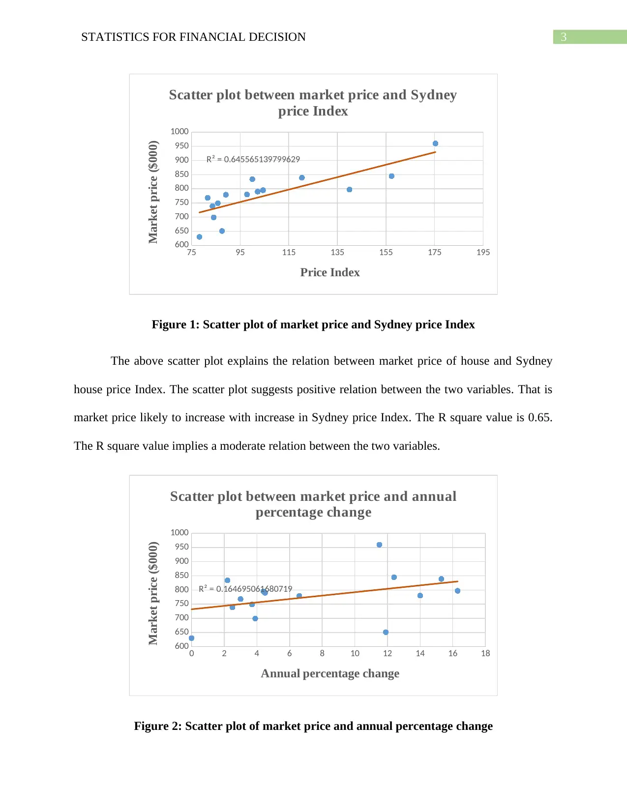
Introduction
The report aims to develop a model that estimates market price of houses depending on
some factors such as Sydney price Index, annual percentage change, land size and age of house.
In Australia especially in capital cities faster increase in house price is the core of housing
affordability crisis (Dufty-Jones 2018). In such a situation it is necessary to estimate market price
of house and its various determinants. The current model considers, market price of houses as a
dependent variable. The four independent variables in the model are Sydney price Index, annual
percentage change, land size and age of house. Market price of house is expressed as thousand
dollars. The Sydney price Index is computed taking base year of 2011-12. The annual change is
the percentage change in house price overtime. Land size is measured in total square meters. Age
of house is expressed as year. The proposed model is estimated taking a sample of 15 years’
period from 2002-03 to 2016-17. The year represents year of built of houses.
Scatter plot
Scatter plot is a useful two-dimensional tool of data visualization explaining relation
between two variables graphically. The dependent variable is plotted on vertical axis while the
independent variable is plotted on the horizontal axis (Chatterjee and Hadi 2015). In the present
model, the dependent variable is market price while the independent variables are Sydney price
Index, annual percentage change in price, land size and age of house. Four different scatter plots
have been constructed to explain the relation between the dependent variable and each of the
independent variables.

3STATISTICS FOR FINANCIAL DECISION
75 95 115 135 155 175 195
600
650
700
750
800
850
900
950
1000
R² = 0.645565139799629
Scatter plot between market price and Sydney
price Index
Price Index
Market price ($000)
Figure 1: Scatter plot of market price and Sydney price Index
The above scatter plot explains the relation between market price of house and Sydney
house price Index. The scatter plot suggests positive relation between the two variables. That is
market price likely to increase with increase in Sydney price Index. The R square value is 0.65.
The R square value implies a moderate relation between the two variables.
0 2 4 6 8 10 12 14 16 18
600
650
700
750
800
850
900
950
1000
R² = 0.164695061680719
Scatter plot between market price and annual
percentage change
Annual percentage change
Market price ($000)
Figure 2: Scatter plot of market price and annual percentage change

4STATISTICS FOR FINANCIAL DECISION
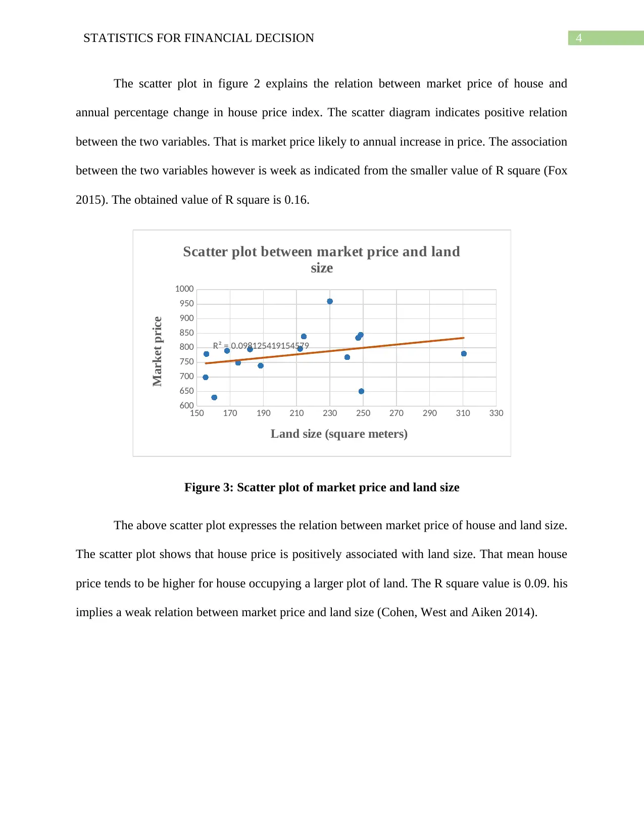
The scatter plot in figure 2 explains the relation between market price of house and
annual percentage change in house price index. The scatter diagram indicates positive relation
between the two variables. That is market price likely to annual increase in price. The association
between the two variables however is week as indicated from the smaller value of R square (Fox
2015). The obtained value of R square is 0.16.
150 170 190 210 230 250 270 290 310 330
600
650
700
750
800
850
900
950
1000
R² = 0.098125419154579
Scatter plot between market price and land
size
Land size (square meters)
Market price
Figure 3: Scatter plot of market price and land size
The above scatter plot expresses the relation between market price of house and land size.
The scatter plot shows that house price is positively associated with land size. That mean house
price tends to be higher for house occupying a larger plot of land. The R square value is 0.09. his
implies a weak relation between market price and land size (Cohen, West and Aiken 2014).

5STATISTICS FOR FINANCIAL DECISION
0 5 10 15 20 25 30 35 40 45 50
600
650
700
750
800
850
900
950
1000
R² = 0.459571351270072
Scatter plot between markert price and age of
house
Age (years)
Market price ($000)
Figure 4: Scatter plot of market price and age of house
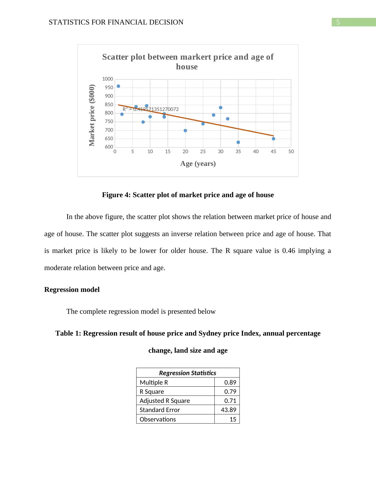
In the above figure, the scatter plot shows the relation between market price of house and
age of house. The scatter plot suggests an inverse relation between price and age of house. That
is market price is likely to be lower for older house. The R square value is 0.46 implying a
moderate relation between price and age.
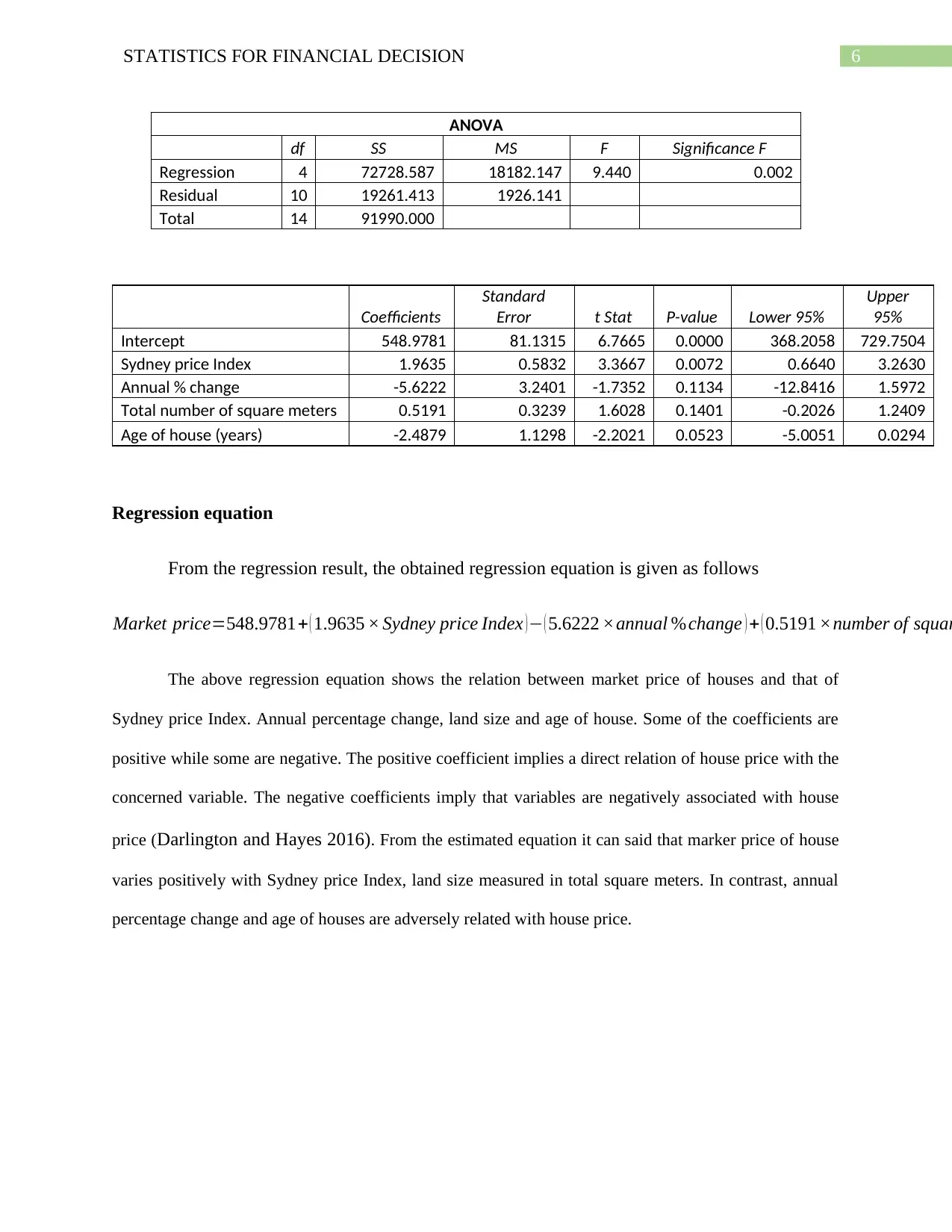
Regression model
The complete regression model is presented below
Table 1: Regression result of house price and Sydney price Index, annual percentage
change, land size and age
Regression Statistics
Multiple R 0.89
R Square 0.79
Adjusted R Square 0.71
Standard Error 43.89
Observations 15

6STATISTICS FOR FINANCIAL DECISION
ANOVA
df SS MS F Significance F
Regression 4 72728.587 18182.147 9.440 0.002
Residual 10 19261.413 1926.141
Total 14 91990.000
Coefficients
Standard
Error t Stat P-value Lower 95%
Upper
95%
Intercept 548.9781 81.1315 6.7665 0.0000 368.2058 729.7504
Sydney price Index 1.9635 0.5832 3.3667 0.0072 0.6640 3.2630
Annual % change -5.6222 3.2401 -1.7352 0.1134 -12.8416 1.5972
Total number of square meters 0.5191 0.3239 1.6028 0.1401 -0.2026 1.2409
Age of house (years) -2.4879 1.1298 -2.2021 0.0523 -5.0051 0.0294
Regression equation
From the regression result, the obtained regression equation is given as follows
Market price=548.9781+ ( 1.9635 × Sydney price Index )− ( 5.6222 ×annual %change ) + ( 0.5191 ×number of squar
The above regression equation shows the relation between market price of houses and that of
Sydney price Index. Annual percentage change, land size and age of house. Some of the coefficients are
positive while some are negative. The positive coefficient implies a direct relation of house price with the
concerned variable. The negative coefficients imply that variables are negatively associated with house
price (Darlington and Hayes 2016). From the estimated equation it can said that marker price of house
varies positively with Sydney price Index, land size measured in total square meters. In contrast, annual
percentage change and age of houses are adversely related with house price.

7STATISTICS FOR FINANCIAL DECISION
Estimated coefficient and their significance
For Sydney price Index the estimated coefficient is 1.9635. Positive sign of the
coefficient implies that house price has a positive relation with Sydney price Index. With
increase in Sydney price Index housing price increases house price increase as well and vice-
versa. More specifically, from the estimated coefficient it can be said that 10 percent increase in
Sydney price Index increases market price of houses by 19 percent. Statistical significance of the
variable can be examined from the associated p value. P value for the regression coefficient is
0.0072. The p value is relatively smaller than 5 percent significance level implying rejection of
null hypothesis of no significant relation between market price and Sydney price Index (Murteira
and Ramalho 2016). Sydney price Index thus is a positive significant determinant of market
price.
In case of annual percentage change the estimated coefficient is -5.6222. Negative
regression coefficient signifies that house price has an inverse relation with annual percentage
change. A higher percentage change therefore leads to decline in market price. More specifically,
from the estimated coefficient it can be said that 1 percent increase in annual percentage
decreases market price of houses by 5.6 percent. Statistical significance of the variable can be
examined from the associated p value. P value for the regression coefficient is 0.1134. The p
value exceeds the 5 percent significance level indicating acceptance of null hypothesis of no
significant relation between market price and annual percentage change. Annual percentage
change thus is not a significant determinant of market price.
For land size measured in total square meters obtained coefficient is 0.5191. Positive sign
of the coefficient implies a positive relation between and land size and market price of houses.
With increase in total square meters area, there is an increase in house price and vice versa. More

8STATISTICS FOR FINANCIAL DECISION
specifically, from the estimated coefficient it can be said that 10 percent increase in land size
increases market price of houses by 5.1 percent (Schober, Boer and Schwarte 2018). Statistical
significance of the variable can be examined from the associated p value. P value for the
regression coefficient is 0.1401. The p value is larger than 5 percent significance level implying
acceptance of null hypothesis of no significant relation between market price and land size. Land
size therefore is not a statistically significant determinant of market price.
The coefficient of ‘age of house’ is -2.4879. Negative coefficient implies that house
varies inversely with age of houses. With increase in age of house housing price, market price
decreases and vice-versa. More specifically, from the estimated coefficient it can be said that 1
percent increase in age of house decreases market price of houses by 2.5 percent. P value for the
regression coefficient is 0.0523. The p value is relatively larger than 5 percent significance level
implying acceptance of null hypothesis of no significant relation between market price and age
of house. Age of houses thus is not a statistically determinant of market price of houses.
Coefficient of determination
In a regression model, the R square value indicates the value of coefficient of
determination. It indicates how much variation in the dependent variable can be explained by the
independent variables together. Coefficient of determination helps to understand explanatory
power of the regression model (Shyu, Grosse and Cleveland 2017). It also determines goodness
of fit of the model. For the obtained regression model, the value of R square is 0.79. The R
square value indicates that Sydney price Index, annual percentage change, land size and age of
house together explains 79 percent variation in market price of house. The value of R square is
close to 1 meaning that the independent variables together account a significant portion of

9STATISTICS FOR FINANCIAL DECISION
variation in market price of houses (Zhang 2017). In all, from the obtained coefficient of
determination, it can be said that the model is a good fit model of estimates.
Confidence interval
For Sydney price Index, the confidence interval for the slope coefficient is (0.6640,
3.2630). The confidence interval implies that, if the same estimation is done with another
sample, we are 95 percent confident that slope coefficient of Sydney price Index lies within this
range. In other words, for 1 percent increase in Sydney price Index, increase in market price
ranges between 0.6640 and 3.2630.
In case of annual percentage change, the confidence interval for the slope coefficient is (-
12.8416, 1.5972). The confidence interval suggests that, if the same estimation is done using
another sample, we are 95 percent confident that slope coefficient of annual percentage change
lies within this range (Piepho 2019). In other words, for 1 percent increase in annual percentage
change, decrease in market price ranges between -12.8416 and 1.5972.
For total number of square meters, the confidence interval for the slope coefficient is (-
0.2026, 1.2409). The confidence interval implies that, if the same estimation is done using
another sample, we are 95 percent confident that slope coefficient of land size varies within this
range. In other words, for 1 percent increase in land size, increase in market price ranges
between -0.2026 and 1.2409.
The 95% confidence interval for age of house is (-5.0051, 0.0294). The confidence
interval implies that, if the same estimation is done using another sample, we are 95 percent
confident that slope coefficient of age of house lies within this range. In other words, for 1

10STATISTICS FOR FINANCIAL DECISION
percent increase in age of house, decrease in market price ranges between -5.0051 and 0.0294
(Draper and Smith 2014).

11STATISTICS FOR FINANCIAL DECISION
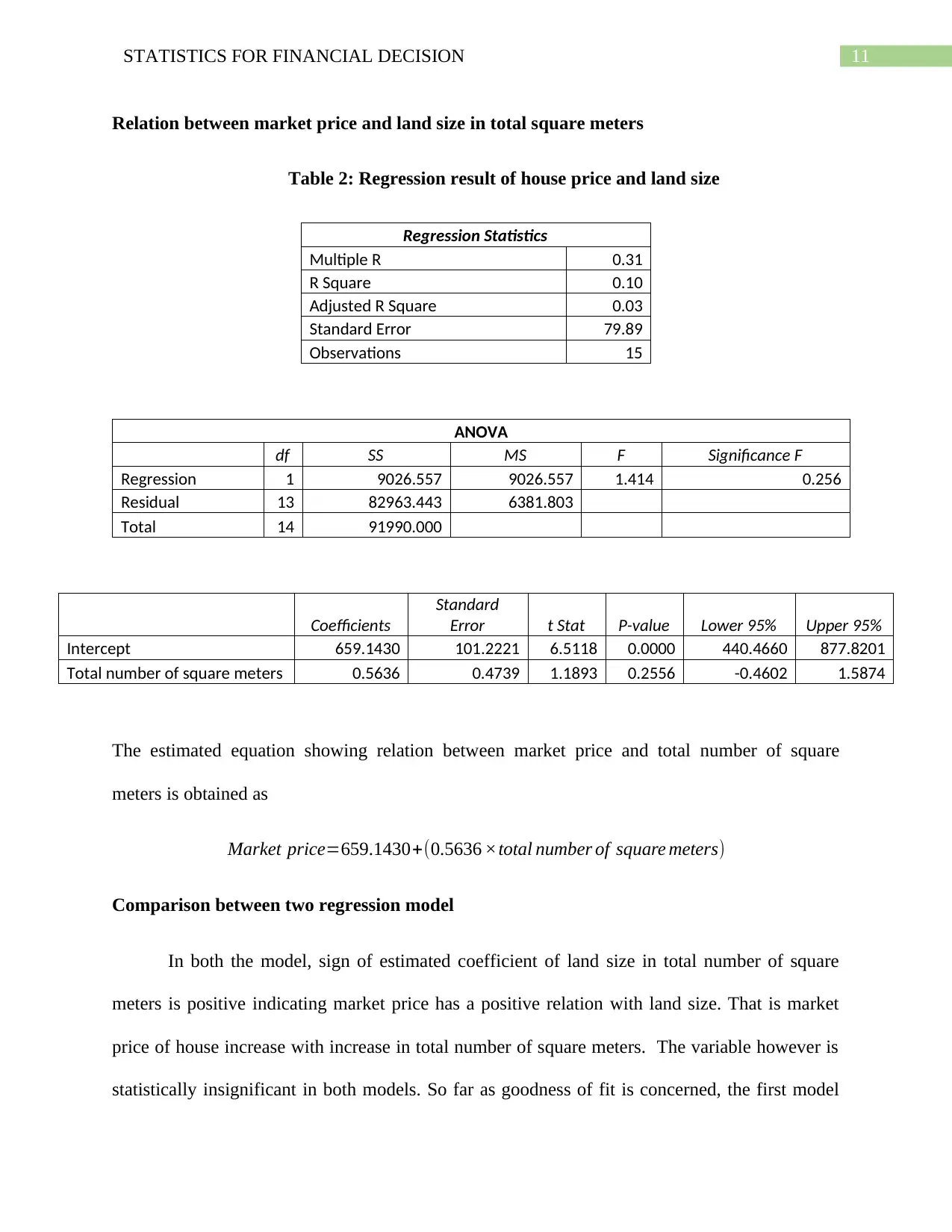
Relation between market price and land size in total square meters
Table 2: Regression result of house price and land size
Regression Statistics
Multiple R 0.31
R Square 0.10
Adjusted R Square 0.03
Standard Error 79.89
Observations 15
ANOVA
df SS MS F Significance F
Regression 1 9026.557 9026.557 1.414 0.256
Residual 13 82963.443 6381.803
Total 14 91990.000
Coefficients
Standard
Error t Stat P-value Lower 95% Upper 95%
Intercept 659.1430 101.2221 6.5118 0.0000 440.4660 877.8201
Total number of square meters 0.5636 0.4739 1.1893 0.2556 -0.4602 1.5874
The estimated equation showing relation between market price and total number of square
meters is obtained as
Market price=659.1430+(0.5636 ×total number of square meters)
Comparison between two regression model
In both the model, sign of estimated coefficient of land size in total number of square
meters is positive indicating market price has a positive relation with land size. That is market
price of house increase with increase in total number of square meters. The variable however is
statistically insignificant in both models. So far as goodness of fit is concerned, the first model