Statistical Analysis and Prediction of House Selling Prices, Sydney
VerifiedAdded on 2023/04/23
|17
|4445
|319
Report
AI Summary
This report presents a statistical analysis of factors influencing house selling prices in Sydney, Australia. The study utilizes a cross-sectional dataset with 28 observations and 10 variables, including selling price, local selling prices, number of bathrooms, site area, living space, garages, rooms, bedrooms, age, and fireplaces. The methodology incorporates descriptive statistics, Pearson correlation tests, and regression analysis to identify relationships between variables. The analysis reveals insights into how various home characteristics impact selling prices. The report includes tables summarizing data, variable descriptions, descriptive statistics, correlations, and regression outputs. The findings are relevant to property owners, real estate brokers, and government authorities involved in the housing market. Data was retrieved from a specified link, and both descriptive and inferential statistics were used to analyze the relationships between variables. The study aims to improve the comprehension of how different home elements affect their moving costs. The results of the Pearson correlation test, along with the regression analysis model, were performed to identify the strength and direction of the relationships between the variables.

PREDICTING SELLING PRICES OF HOUSES
Statistics
Student Name:
Student Number:
Date: 14th January 2019
Statistics
Student Name:
Student Number:
Date: 14th January 2019
Paraphrase This Document
Need a fresh take? Get an instant paraphrase of this document with our AI Paraphraser
Table of Contents
Introduction......................................................................................................................................3
Methodology....................................................................................................................................3
Data..................................................................................................................................................4
Description of the variables.........................................................................................................6
Data Analysis...................................................................................................................................6
Descriptive Statistics....................................................................................................................6
Measure of association.................................................................................................................8
Regression analysis....................................................................................................................10
Conclusion.....................................................................................................................................13
List of tables
Table 1: Dataset...............................................................................................................................4
Table 2: Variable names..................................................................................................................5
Table 3: Description of variables.....................................................................................................6
Table 4: Descriptive statistics..........................................................................................................7
Table 5: Correlations.......................................................................................................................8
Table 6: SUMMARY OUTPUT....................................................................................................10
Table 7: ANOVA...........................................................................................................................11
Table 8: Coefficients table.............................................................................................................11
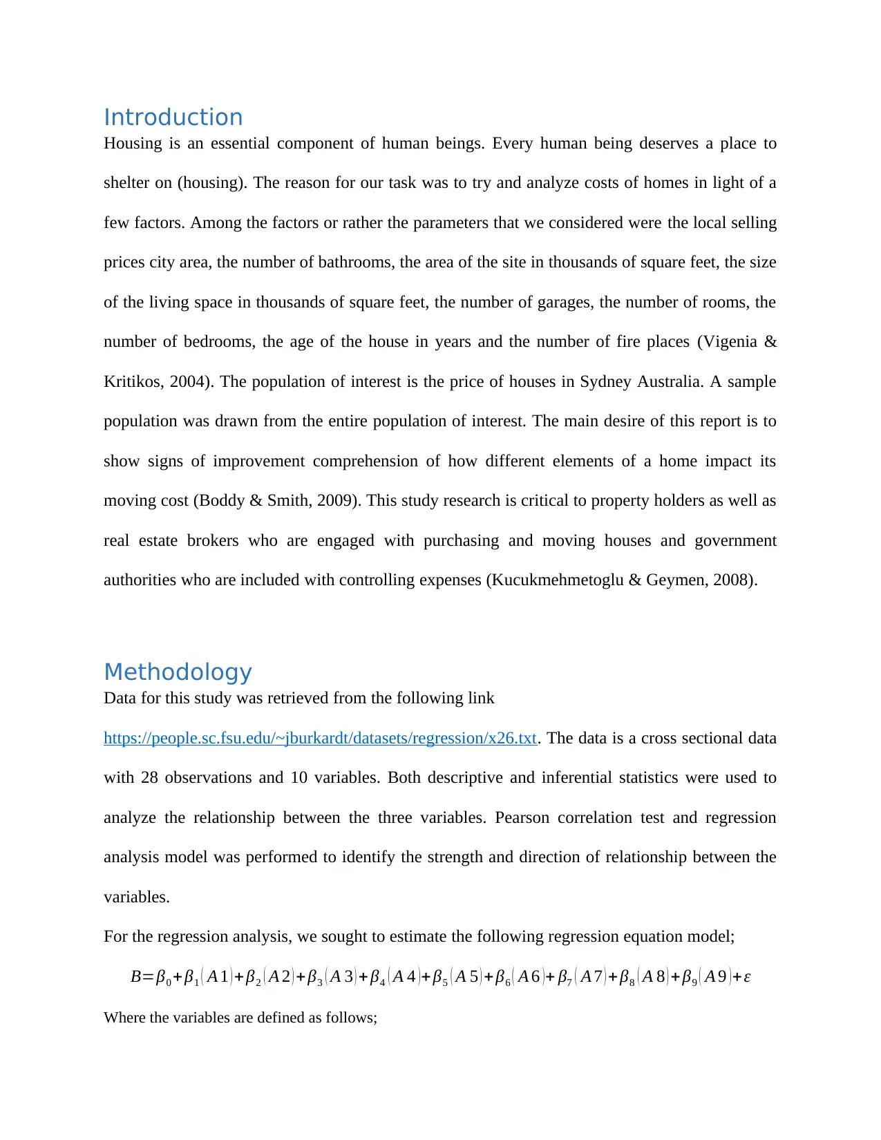
Introduction
Housing is an essential component of human beings. Every human being deserves a place to
shelter on (housing). The reason for our task was to try and analyze costs of homes in light of a
few factors. Among the factors or rather the parameters that we considered were the local selling
prices city area, the number of bathrooms, the area of the site in thousands of square feet, the size
of the living space in thousands of square feet, the number of garages, the number of rooms, the
number of bedrooms, the age of the house in years and the number of fire places (Vigenia &
Kritikos, 2004). The population of interest is the price of houses in Sydney Australia. A sample
population was drawn from the entire population of interest. The main desire of this report is to
show signs of improvement comprehension of how different elements of a home impact its
moving cost (Boddy & Smith, 2009). This study research is critical to property holders as well as
real estate brokers who are engaged with purchasing and moving houses and government
authorities who are included with controlling expenses (Kucukmehmetoglu & Geymen, 2008).
Methodology
Data for this study was retrieved from the following link
https://people.sc.fsu.edu/~jburkardt/datasets/regression/x26.txt. The data is a cross sectional data
with 28 observations and 10 variables. Both descriptive and inferential statistics were used to
analyze the relationship between the three variables. Pearson correlation test and regression
analysis model was performed to identify the strength and direction of relationship between the
variables.
For the regression analysis, we sought to estimate the following regression equation model;
B=β0 + β1 ( A 1 ) + β2 ( A 2 ) + β3 ( A 3 ) + β4 ( A 4 ) + β5 ( A 5 ) + β6 ( A 6 ) + β7 ( A 7 ) + β8 ( A 8 ) + β9 ( A 9 ) +ε
Where the variables are defined as follows;
⊘ This is a preview!⊘
Do you want full access?
Subscribe today to unlock all pages.
Trusted by 1+ million students worldwide
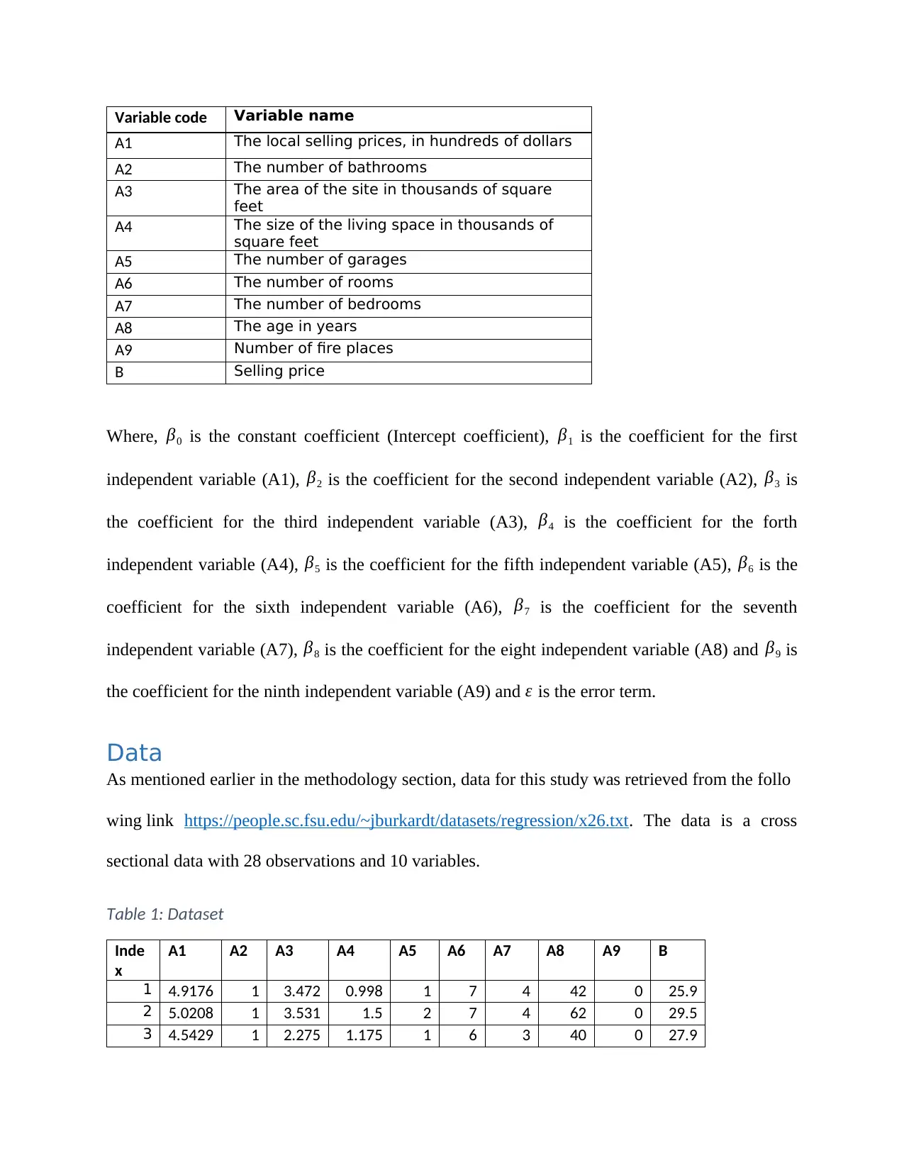
Variable code Variable name
A1 The local selling prices, in hundreds of dollars
A2 The number of bathrooms
A3 The area of the site in thousands of square
feet
A4 The size of the living space in thousands of
square feet
A5 The number of garages
A6 The number of rooms
A7 The number of bedrooms
A8 The age in years
A9 Number of fire places
B Selling price
Where, β0 is the constant coefficient (Intercept coefficient), β1 is the coefficient for the first
independent variable (A1), β2 is the coefficient for the second independent variable (A2), β3 is
the coefficient for the third independent variable (A3), β4 is the coefficient for the forth
independent variable (A4), β5 is the coefficient for the fifth independent variable (A5), β6 is the
coefficient for the sixth independent variable (A6), β7 is the coefficient for the seventh
independent variable (A7), β8 is the coefficient for the eight independent variable (A8) and β9 is
the coefficient for the ninth independent variable (A9) and ε is the error term.
Data
As mentioned earlier in the methodology section, data for this study was retrieved from the follo
wing link https://people.sc.fsu.edu/~jburkardt/datasets/regression/x26.txt. The data is a cross
sectional data with 28 observations and 10 variables.
Table 1: Dataset
Inde
x
A1 A2 A3 A4 A5 A6 A7 A8 A9 B
1 4.9176 1 3.472 0.998 1 7 4 42 0 25.9
2 5.0208 1 3.531 1.5 2 7 4 62 0 29.5
3 4.5429 1 2.275 1.175 1 6 3 40 0 27.9
Paraphrase This Document
Need a fresh take? Get an instant paraphrase of this document with our AI Paraphraser
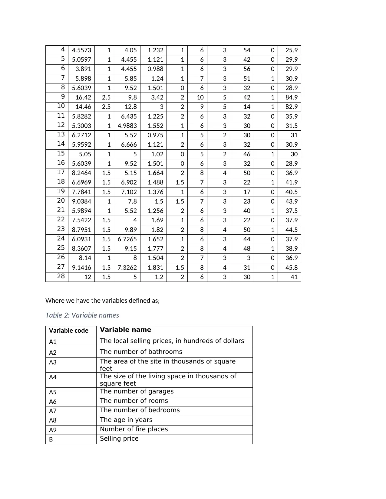
4 4.5573 1 4.05 1.232 1 6 3 54 0 25.9
5 5.0597 1 4.455 1.121 1 6 3 42 0 29.9
6 3.891 1 4.455 0.988 1 6 3 56 0 29.9
7 5.898 1 5.85 1.24 1 7 3 51 1 30.9
8 5.6039 1 9.52 1.501 0 6 3 32 0 28.9
9 16.42 2.5 9.8 3.42 2 10 5 42 1 84.9
10 14.46 2.5 12.8 3 2 9 5 14 1 82.9
11 5.8282 1 6.435 1.225 2 6 3 32 0 35.9
12 5.3003 1 4.9883 1.552 1 6 3 30 0 31.5
13 6.2712 1 5.52 0.975 1 5 2 30 0 31
14 5.9592 1 6.666 1.121 2 6 3 32 0 30.9
15 5.05 1 5 1.02 0 5 2 46 1 30
16 5.6039 1 9.52 1.501 0 6 3 32 0 28.9
17 8.2464 1.5 5.15 1.664 2 8 4 50 0 36.9
18 6.6969 1.5 6.902 1.488 1.5 7 3 22 1 41.9
19 7.7841 1.5 7.102 1.376 1 6 3 17 0 40.5
20 9.0384 1 7.8 1.5 1.5 7 3 23 0 43.9
21 5.9894 1 5.52 1.256 2 6 3 40 1 37.5
22 7.5422 1.5 4 1.69 1 6 3 22 0 37.9
23 8.7951 1.5 9.89 1.82 2 8 4 50 1 44.5
24 6.0931 1.5 6.7265 1.652 1 6 3 44 0 37.9
25 8.3607 1.5 9.15 1.777 2 8 4 48 1 38.9
26 8.14 1 8 1.504 2 7 3 3 0 36.9
27 9.1416 1.5 7.3262 1.831 1.5 8 4 31 0 45.8
28 12 1.5 5 1.2 2 6 3 30 1 41
Where we have the variables defined as;
Table 2: Variable names
Variable code Variable name
A1 The local selling prices, in hundreds of dollars
A2 The number of bathrooms
A3 The area of the site in thousands of square
feet
A4 The size of the living space in thousands of
square feet
A5 The number of garages
A6 The number of rooms
A7 The number of bedrooms
A8 The age in years
A9 Number of fire places
B Selling price
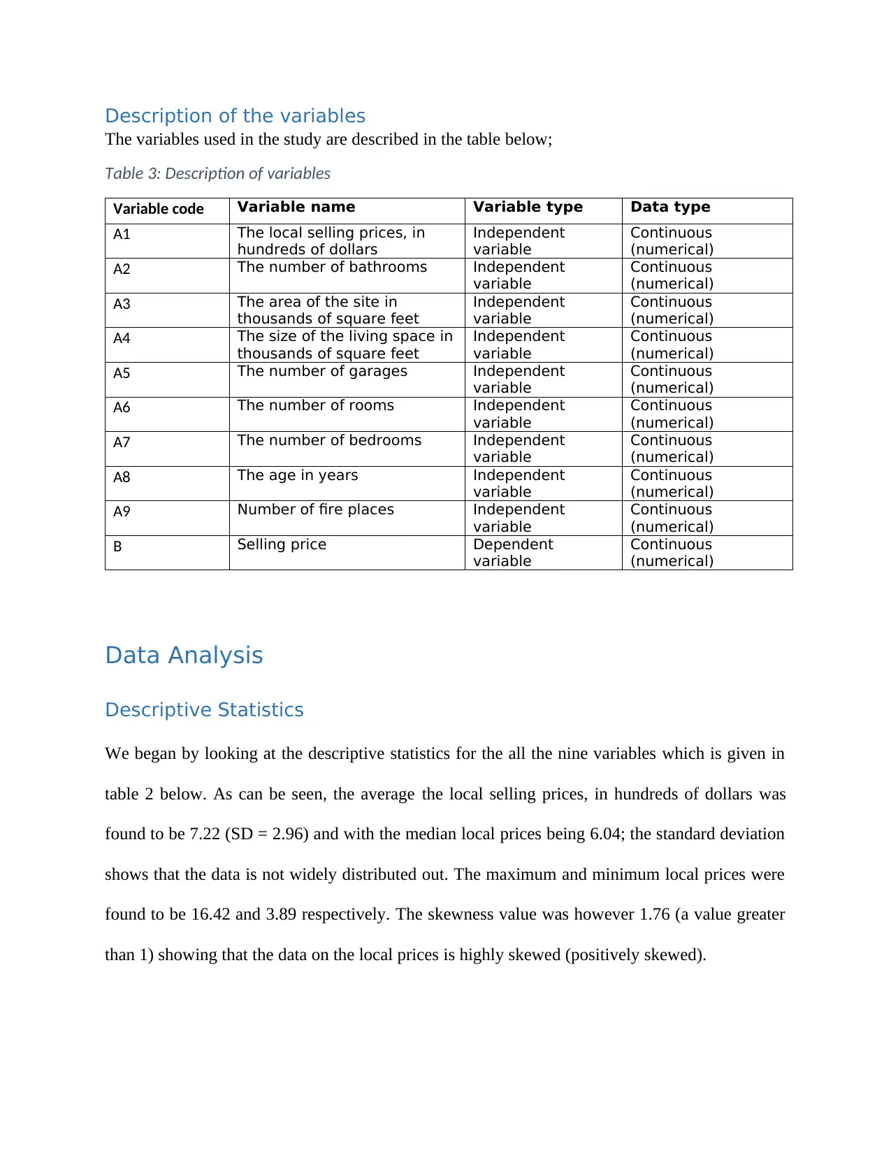
Description of the variables
The variables used in the study are described in the table below;
Table 3: Description of variables
Variable code Variable name Variable type Data type
A1 The local selling prices, in
hundreds of dollars
Independent
variable
Continuous
(numerical)
A2 The number of bathrooms Independent
variable
Continuous
(numerical)
A3 The area of the site in
thousands of square feet
Independent
variable
Continuous
(numerical)
A4 The size of the living space in
thousands of square feet
Independent
variable
Continuous
(numerical)
A5 The number of garages Independent
variable
Continuous
(numerical)
A6 The number of rooms Independent
variable
Continuous
(numerical)
A7 The number of bedrooms Independent
variable
Continuous
(numerical)
A8 The age in years Independent
variable
Continuous
(numerical)
A9 Number of fire places Independent
variable
Continuous
(numerical)
B Selling price Dependent
variable
Continuous
(numerical)
Data Analysis
Descriptive Statistics
We began by looking at the descriptive statistics for the all the nine variables which is given in
table 2 below. As can be seen, the average the local selling prices, in hundreds of dollars was
found to be 7.22 (SD = 2.96) and with the median local prices being 6.04; the standard deviation
shows that the data is not widely distributed out. The maximum and minimum local prices were
found to be 16.42 and 3.89 respectively. The skewness value was however 1.76 (a value greater
than 1) showing that the data on the local prices is highly skewed (positively skewed).
⊘ This is a preview!⊘
Do you want full access?
Subscribe today to unlock all pages.
Trusted by 1+ million students worldwide
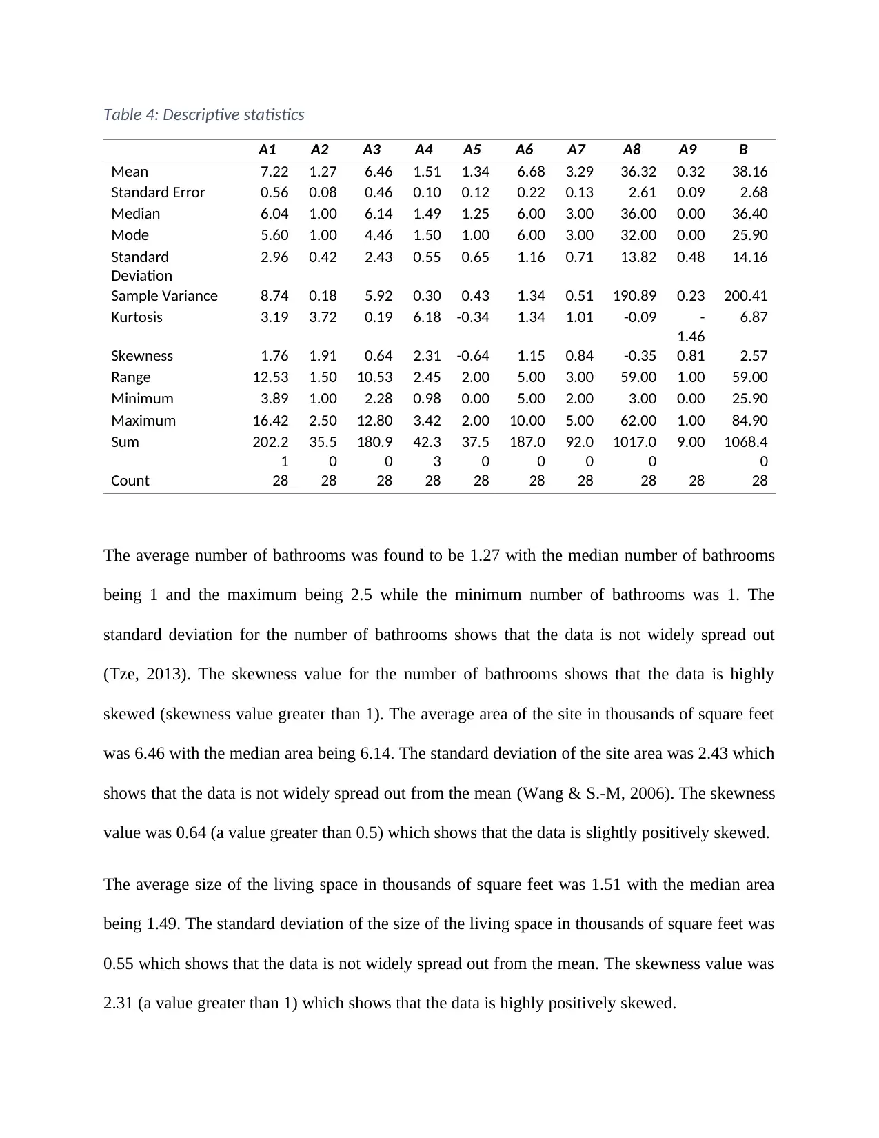
Table 4: Descriptive statistics
A1 A2 A3 A4 A5 A6 A7 A8 A9 B
Mean 7.22 1.27 6.46 1.51 1.34 6.68 3.29 36.32 0.32 38.16
Standard Error 0.56 0.08 0.46 0.10 0.12 0.22 0.13 2.61 0.09 2.68
Median 6.04 1.00 6.14 1.49 1.25 6.00 3.00 36.00 0.00 36.40
Mode 5.60 1.00 4.46 1.50 1.00 6.00 3.00 32.00 0.00 25.90
Standard
Deviation
2.96 0.42 2.43 0.55 0.65 1.16 0.71 13.82 0.48 14.16
Sample Variance 8.74 0.18 5.92 0.30 0.43 1.34 0.51 190.89 0.23 200.41
Kurtosis 3.19 3.72 0.19 6.18 -0.34 1.34 1.01 -0.09 -
1.46
6.87
Skewness 1.76 1.91 0.64 2.31 -0.64 1.15 0.84 -0.35 0.81 2.57
Range 12.53 1.50 10.53 2.45 2.00 5.00 3.00 59.00 1.00 59.00
Minimum 3.89 1.00 2.28 0.98 0.00 5.00 2.00 3.00 0.00 25.90
Maximum 16.42 2.50 12.80 3.42 2.00 10.00 5.00 62.00 1.00 84.90
Sum 202.2
1
35.5
0
180.9
0
42.3
3
37.5
0
187.0
0
92.0
0
1017.0
0
9.00 1068.4
0
Count 28 28 28 28 28 28 28 28 28 28
The average number of bathrooms was found to be 1.27 with the median number of bathrooms
being 1 and the maximum being 2.5 while the minimum number of bathrooms was 1. The
standard deviation for the number of bathrooms shows that the data is not widely spread out
(Tze, 2013). The skewness value for the number of bathrooms shows that the data is highly
skewed (skewness value greater than 1). The average area of the site in thousands of square feet
was 6.46 with the median area being 6.14. The standard deviation of the site area was 2.43 which
shows that the data is not widely spread out from the mean (Wang & S.-M, 2006). The skewness
value was 0.64 (a value greater than 0.5) which shows that the data is slightly positively skewed.
The average size of the living space in thousands of square feet was 1.51 with the median area
being 1.49. The standard deviation of the size of the living space in thousands of square feet was
0.55 which shows that the data is not widely spread out from the mean. The skewness value was
2.31 (a value greater than 1) which shows that the data is highly positively skewed.
Paraphrase This Document
Need a fresh take? Get an instant paraphrase of this document with our AI Paraphraser
The average number of garages was 1.34 with the median area being 1.25. The standard
deviation of the number of garages was 0.65 which shows that the data is not widely spread out
from the mean. The skewness value was -0.64 (a value greater than -0.5) which shows that the
data is slightly negatively skewed.
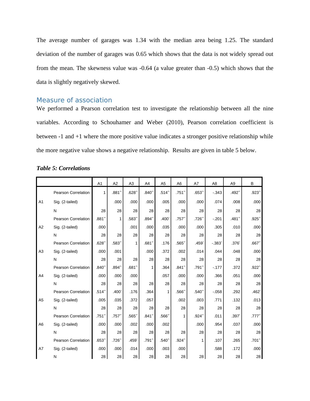
Measure of association
We performed a Pearson correlation test to investigate the relationship between all the nine
variables. According to Schouhamer and Weber (2010), Pearson correlation coefficient is
between -1 and +1 where the more positive value indicates a stronger positive relationship while
the more negative value shows a negative relationship. Results are given in table 5 below.
Table 5: Correlations
A1 A2 A3 A4 A5 A6 A7 A8 A9 B
A1
Pearson Correlation 1 .881** .628** .840** .514** .751** .653** -.343 .492** .923**
Sig. (2-tailed) .000 .000 .000 .005 .000 .000 .074 .008 .000
N 28 28 28 28 28 28 28 28 28 28
A2
Pearson Correlation .881** 1 .583** .894** .400* .757** .726** -.201 .481** .925**
Sig. (2-tailed) .000 .001 .000 .035 .000 .000 .305 .010 .000
N 28 28 28 28 28 28 28 28 28 28
A3
Pearson Correlation .628** .583** 1 .681** .176 .565** .459* -.383* .376* .667**
Sig. (2-tailed) .000 .001 .000 .372 .002 .014 .044 .048 .000
N 28 28 28 28 28 28 28 28 28 28
A4
Pearson Correlation .840** .894** .681** 1 .364 .841** .791** -.177 .372 .922**
Sig. (2-tailed) .000 .000 .000 .057 .000 .000 .366 .051 .000
N 28 28 28 28 28 28 28 28 28 28
A5
Pearson Correlation .514** .400* .176 .364 1 .566** .540** -.058 .292 .462*
Sig. (2-tailed) .005 .035 .372 .057 .002 .003 .771 .132 .013
N 28 28 28 28 28 28 28 28 28 28
A6
Pearson Correlation .751** .757** .565** .841** .566** 1 .924** .011 .397* .777**
Sig. (2-tailed) .000 .000 .002 .000 .002 .000 .954 .037 .000
N 28 28 28 28 28 28 28 28 28 28
A7
Pearson Correlation .653** .726** .459* .791** .540** .924** 1 .107 .265 .701**
Sig. (2-tailed) .000 .000 .014 .000 .003 .000 .588 .172 .000
N 28 28 28 28 28 28 28 28 28 28
deviation of the number of garages was 0.65 which shows that the data is not widely spread out
from the mean. The skewness value was -0.64 (a value greater than -0.5) which shows that the
data is slightly negatively skewed.
Measure of association
We performed a Pearson correlation test to investigate the relationship between all the nine
variables. According to Schouhamer and Weber (2010), Pearson correlation coefficient is
between -1 and +1 where the more positive value indicates a stronger positive relationship while
the more negative value shows a negative relationship. Results are given in table 5 below.
Table 5: Correlations
A1 A2 A3 A4 A5 A6 A7 A8 A9 B
A1
Pearson Correlation 1 .881** .628** .840** .514** .751** .653** -.343 .492** .923**
Sig. (2-tailed) .000 .000 .000 .005 .000 .000 .074 .008 .000
N 28 28 28 28 28 28 28 28 28 28
A2
Pearson Correlation .881** 1 .583** .894** .400* .757** .726** -.201 .481** .925**
Sig. (2-tailed) .000 .001 .000 .035 .000 .000 .305 .010 .000
N 28 28 28 28 28 28 28 28 28 28
A3
Pearson Correlation .628** .583** 1 .681** .176 .565** .459* -.383* .376* .667**
Sig. (2-tailed) .000 .001 .000 .372 .002 .014 .044 .048 .000
N 28 28 28 28 28 28 28 28 28 28
A4
Pearson Correlation .840** .894** .681** 1 .364 .841** .791** -.177 .372 .922**
Sig. (2-tailed) .000 .000 .000 .057 .000 .000 .366 .051 .000
N 28 28 28 28 28 28 28 28 28 28
A5
Pearson Correlation .514** .400* .176 .364 1 .566** .540** -.058 .292 .462*
Sig. (2-tailed) .005 .035 .372 .057 .002 .003 .771 .132 .013
N 28 28 28 28 28 28 28 28 28 28
A6
Pearson Correlation .751** .757** .565** .841** .566** 1 .924** .011 .397* .777**
Sig. (2-tailed) .000 .000 .002 .000 .002 .000 .954 .037 .000
N 28 28 28 28 28 28 28 28 28 28
A7
Pearson Correlation .653** .726** .459* .791** .540** .924** 1 .107 .265 .701**
Sig. (2-tailed) .000 .000 .014 .000 .003 .000 .588 .172 .000
N 28 28 28 28 28 28 28 28 28 28
A8
Pearson Correlation -.343 -.201 -.383* -.177 -.058 .011 .107 1 .091 -.299
Sig. (2-tailed) .074 .305 .044 .366 .771 .954 .588 .646 .122
N 28 28 28 28 28 28 28 28 28 28
A9
Pearson Correlation .492** .481** .376* .372 .292 .397* .265 .091 1 .490**
Sig. (2-tailed) .008 .010 .048 .051 .132 .037 .172 .646 .008
N 28 28 28 28 28 28 28 28 28 28
B Pearson Correlation .923** .925** .667** .922** .462* .777** .701** -.299 .490** 1
Sig. (2-tailed) .000 .000 .000 .000 .013 .000 .000 .122 .008
N 28 28 28 28 28 28 28 28 28 28
**. Correlation is significant at the 0.01 level (2-tailed).
*. Correlation is significant at the 0.05 level (2-tailed).
The above results shows that there is a significant relationship between the expected house prices
and eight of the nine independent variables. The only variable that did not have any significant
relationship with the dependent variable (House prices) is the age of the house in years. The
number of bathrooms had the highest relationship with the dependent variable (selling price).
The correlation coefficient was found to be 0.925 with the p-value of 0.000.
There was also a very strong relationship between the local selling prices, in hundreds of dollars
(A1) and the selling price (B) where the correlation coefficient was found to be 0.923 (p =
0.000). The correlation coefficient between the area of the site in thousands of square feet (A3)
and the selling price (B) was 0.922 (p = 0.000).
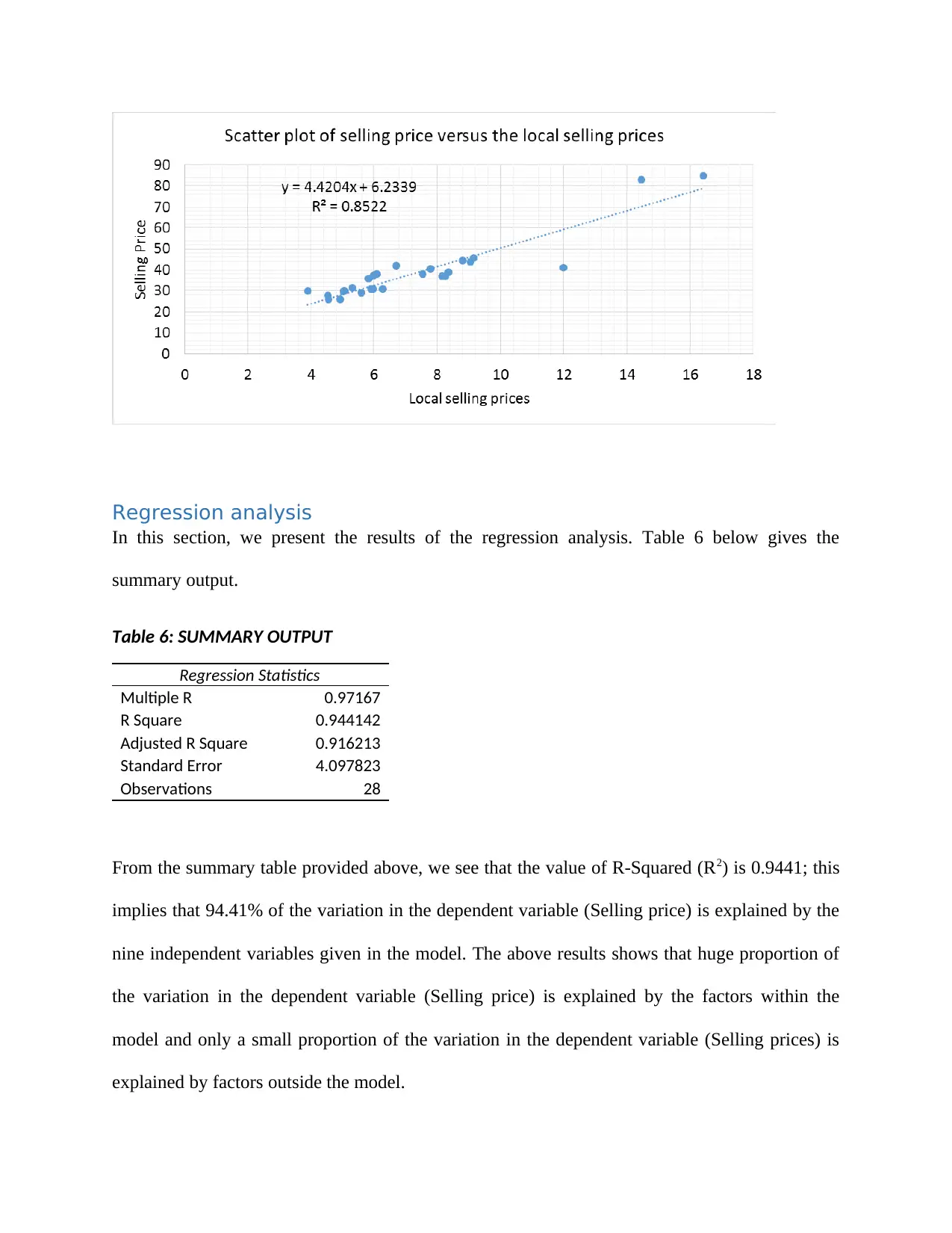
Scatter plot
The scatter plot below is that of the selling price versus the local selling prices (Allen, et al.,
2008). As can be seen, the scatter plot further confirms that there is a strong positive relationship
between local selling price (A1) and the selling prices of the houses (B).
Pearson Correlation -.343 -.201 -.383* -.177 -.058 .011 .107 1 .091 -.299
Sig. (2-tailed) .074 .305 .044 .366 .771 .954 .588 .646 .122
N 28 28 28 28 28 28 28 28 28 28
A9
Pearson Correlation .492** .481** .376* .372 .292 .397* .265 .091 1 .490**
Sig. (2-tailed) .008 .010 .048 .051 .132 .037 .172 .646 .008
N 28 28 28 28 28 28 28 28 28 28
B Pearson Correlation .923** .925** .667** .922** .462* .777** .701** -.299 .490** 1
Sig. (2-tailed) .000 .000 .000 .000 .013 .000 .000 .122 .008
N 28 28 28 28 28 28 28 28 28 28
**. Correlation is significant at the 0.01 level (2-tailed).
*. Correlation is significant at the 0.05 level (2-tailed).
The above results shows that there is a significant relationship between the expected house prices
and eight of the nine independent variables. The only variable that did not have any significant
relationship with the dependent variable (House prices) is the age of the house in years. The
number of bathrooms had the highest relationship with the dependent variable (selling price).
The correlation coefficient was found to be 0.925 with the p-value of 0.000.
There was also a very strong relationship between the local selling prices, in hundreds of dollars
(A1) and the selling price (B) where the correlation coefficient was found to be 0.923 (p =
0.000). The correlation coefficient between the area of the site in thousands of square feet (A3)
and the selling price (B) was 0.922 (p = 0.000).
Scatter plot
The scatter plot below is that of the selling price versus the local selling prices (Allen, et al.,
2008). As can be seen, the scatter plot further confirms that there is a strong positive relationship
between local selling price (A1) and the selling prices of the houses (B).
⊘ This is a preview!⊘
Do you want full access?
Subscribe today to unlock all pages.
Trusted by 1+ million students worldwide
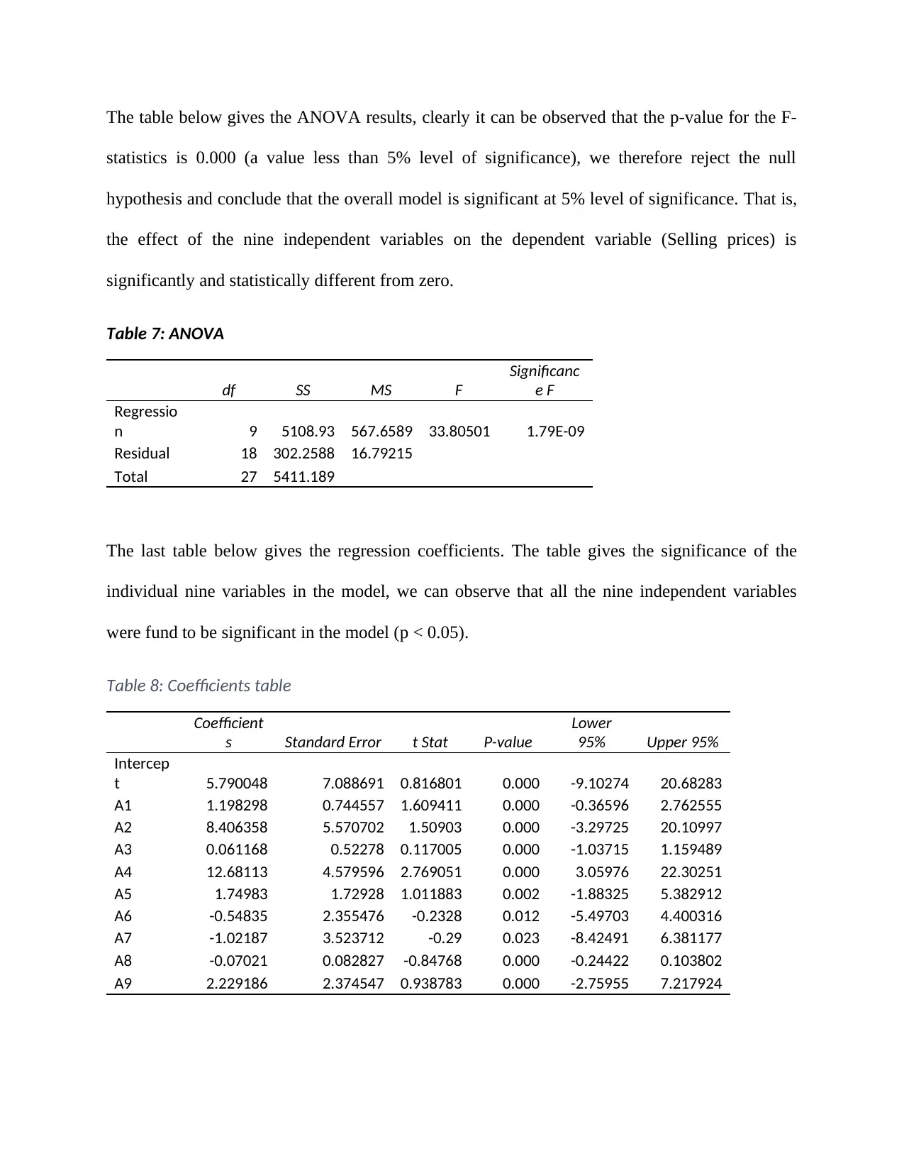
Regression analysis
In this section, we present the results of the regression analysis. Table 6 below gives the
summary output.
Table 6: SUMMARY OUTPUT
Regression Statistics
Multiple R 0.97167
R Square 0.944142
Adjusted R Square 0.916213
Standard Error 4.097823
Observations 28
From the summary table provided above, we see that the value of R-Squared (R2) is 0.9441; this
implies that 94.41% of the variation in the dependent variable (Selling price) is explained by the
nine independent variables given in the model. The above results shows that huge proportion of
the variation in the dependent variable (Selling price) is explained by the factors within the
model and only a small proportion of the variation in the dependent variable (Selling prices) is
explained by factors outside the model.
Paraphrase This Document
Need a fresh take? Get an instant paraphrase of this document with our AI Paraphraser
The table below gives the ANOVA results, clearly it can be observed that the p-value for the F-
statistics is 0.000 (a value less than 5% level of significance), we therefore reject the null
hypothesis and conclude that the overall model is significant at 5% level of significance. That is,
the effect of the nine independent variables on the dependent variable (Selling prices) is
significantly and statistically different from zero.
Table 7: ANOVA
df SS MS F
Significanc
e F
Regressio
n 9 5108.93 567.6589 33.80501 1.79E-09
Residual 18 302.2588 16.79215
Total 27 5411.189
The last table below gives the regression coefficients. The table gives the significance of the
individual nine variables in the model, we can observe that all the nine independent variables
were fund to be significant in the model (p < 0.05).
Table 8: Coefficients table
Coefficient
s Standard Error t Stat P-value
Lower
95% Upper 95%
Intercep
t 5.790048 7.088691 0.816801 0.000 -9.10274 20.68283
A1 1.198298 0.744557 1.609411 0.000 -0.36596 2.762555
A2 8.406358 5.570702 1.50903 0.000 -3.29725 20.10997
A3 0.061168 0.52278 0.117005 0.000 -1.03715 1.159489
A4 12.68113 4.579596 2.769051 0.000 3.05976 22.30251
A5 1.74983 1.72928 1.011883 0.002 -1.88325 5.382912
A6 -0.54835 2.355476 -0.2328 0.012 -5.49703 4.400316
A7 -1.02187 3.523712 -0.29 0.023 -8.42491 6.381177
A8 -0.07021 0.082827 -0.84768 0.000 -0.24422 0.103802
A9 2.229186 2.374547 0.938783 0.000 -2.75955 7.217924
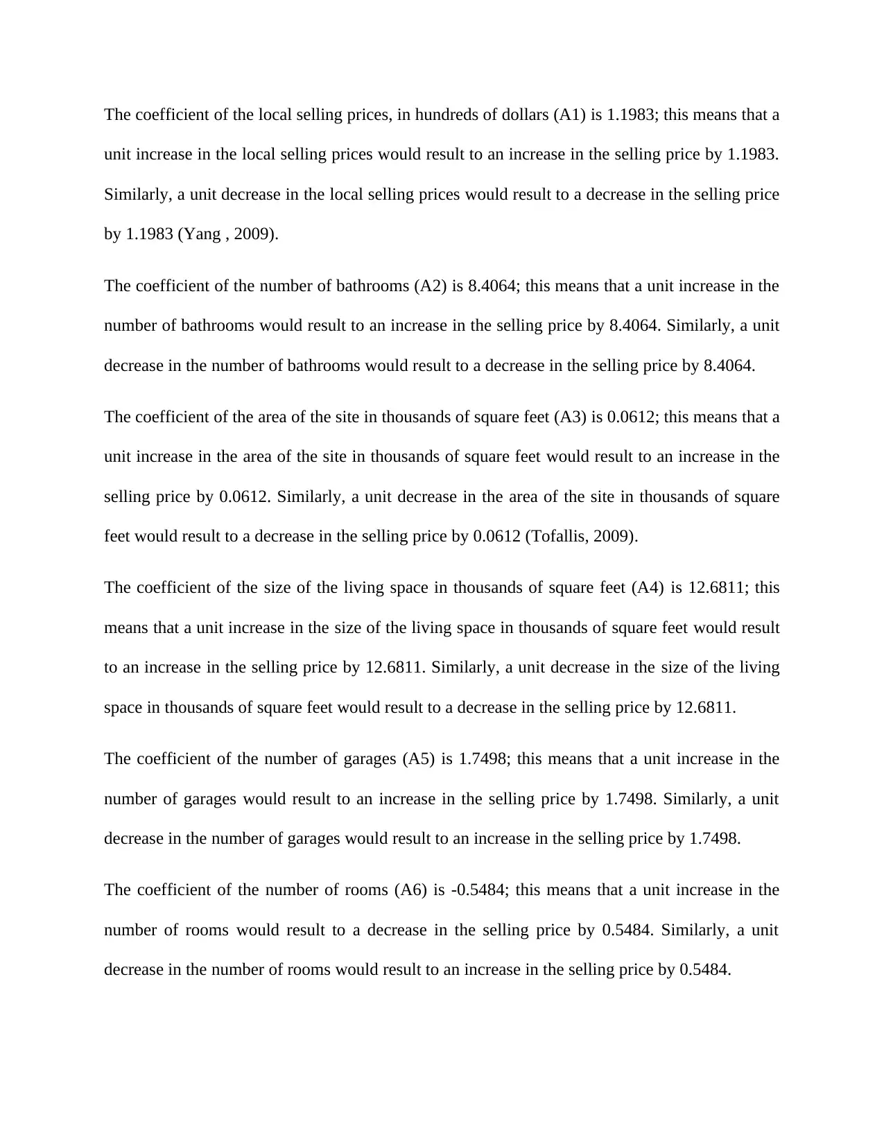
The coefficient of the local selling prices, in hundreds of dollars (A1) is 1.1983; this means that a
unit increase in the local selling prices would result to an increase in the selling price by 1.1983.
Similarly, a unit decrease in the local selling prices would result to a decrease in the selling price
by 1.1983 (Yang , 2009).
The coefficient of the number of bathrooms (A2) is 8.4064; this means that a unit increase in the
number of bathrooms would result to an increase in the selling price by 8.4064. Similarly, a unit
decrease in the number of bathrooms would result to a decrease in the selling price by 8.4064.
The coefficient of the area of the site in thousands of square feet (A3) is 0.0612; this means that a
unit increase in the area of the site in thousands of square feet would result to an increase in the
selling price by 0.0612. Similarly, a unit decrease in the area of the site in thousands of square
feet would result to a decrease in the selling price by 0.0612 (Tofallis, 2009).
The coefficient of the size of the living space in thousands of square feet (A4) is 12.6811; this
means that a unit increase in the size of the living space in thousands of square feet would result
to an increase in the selling price by 12.6811. Similarly, a unit decrease in the size of the living
space in thousands of square feet would result to a decrease in the selling price by 12.6811.
The coefficient of the number of garages (A5) is 1.7498; this means that a unit increase in the
number of garages would result to an increase in the selling price by 1.7498. Similarly, a unit
decrease in the number of garages would result to an increase in the selling price by 1.7498.
The coefficient of the number of rooms (A6) is -0.5484; this means that a unit increase in the
number of rooms would result to a decrease in the selling price by 0.5484. Similarly, a unit
decrease in the number of rooms would result to an increase in the selling price by 0.5484.
⊘ This is a preview!⊘
Do you want full access?
Subscribe today to unlock all pages.
Trusted by 1+ million students worldwide
1 out of 17
Related Documents


Your All-in-One AI-Powered Toolkit for Academic Success.
+13062052269
info@desklib.com
Available 24*7 on WhatsApp / Email
![[object Object]](/_next/static/media/star-bottom.7253800d.svg)
Unlock your academic potential
Copyright © 2020–2026 A2Z Services. All Rights Reserved. Developed and managed by ZUCOL.