Statistical Hydrology Project: Bridge Design and Flood Analysis Report

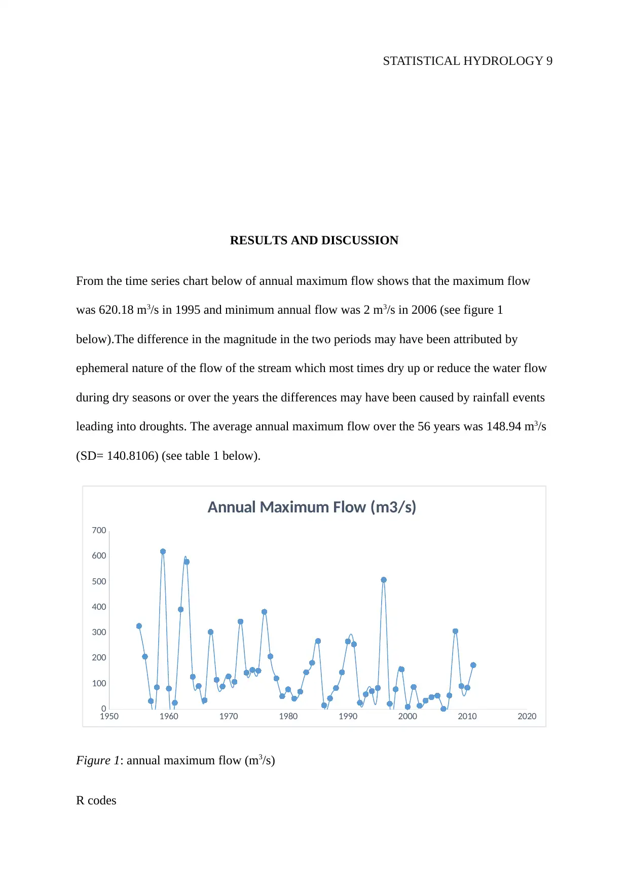
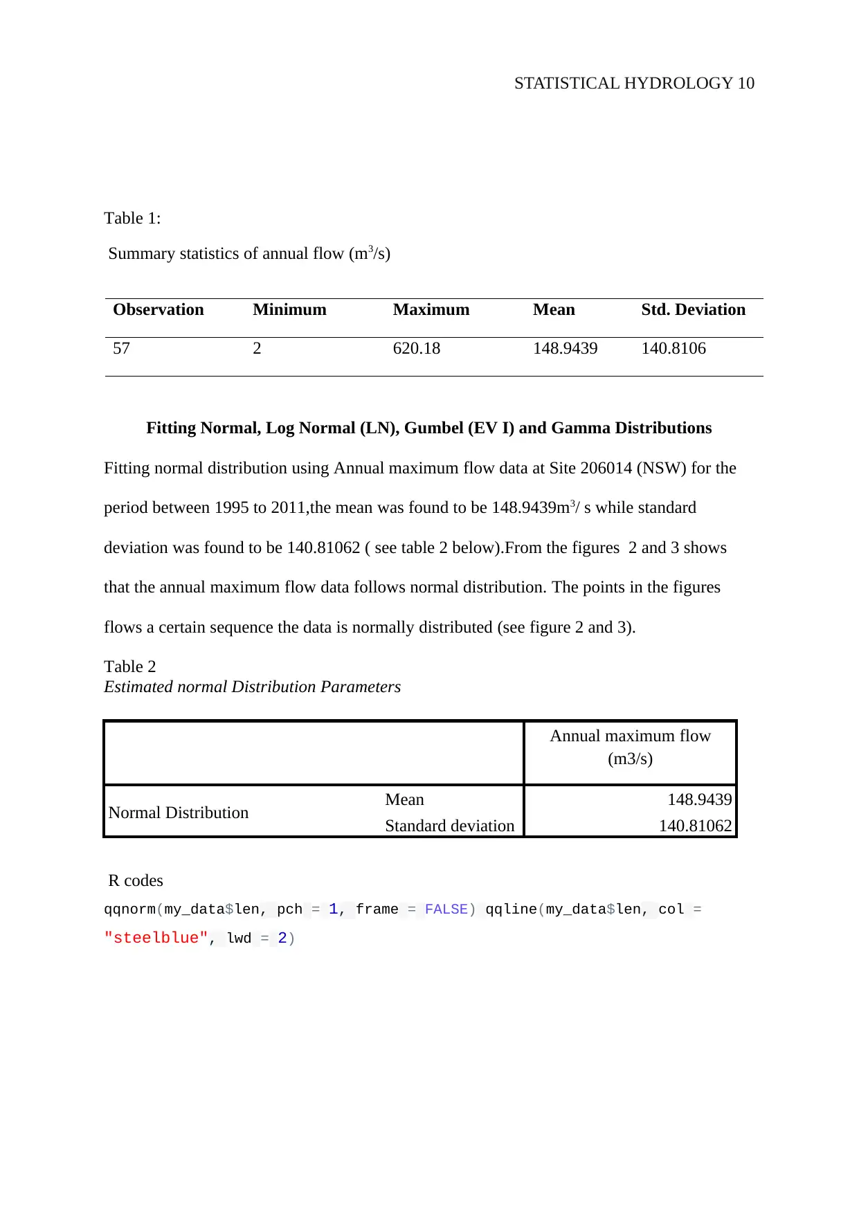
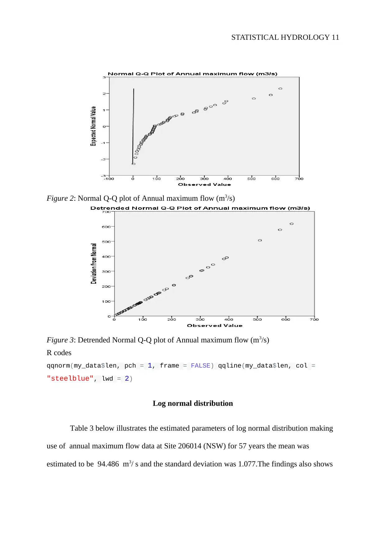
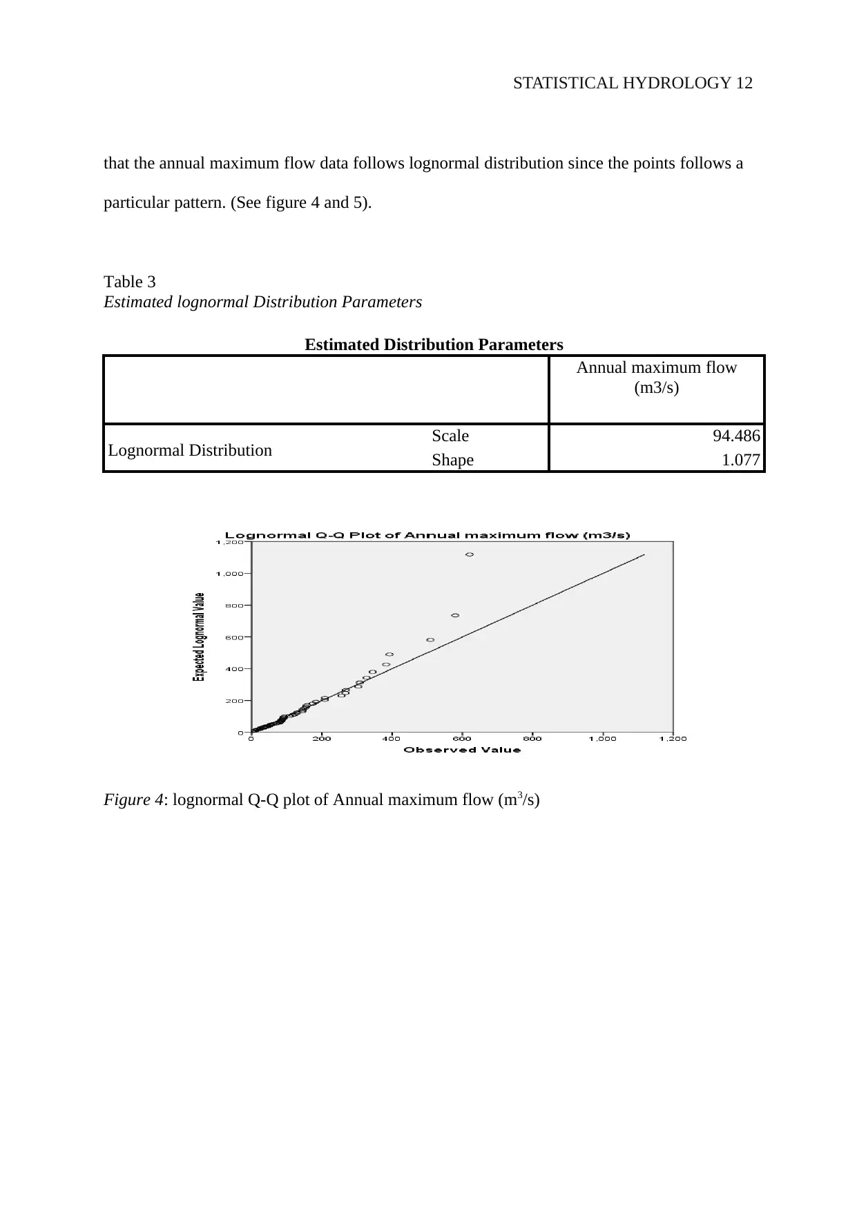
This project is a comprehensive statistical hydrology analysis focused on determining a suitable flood discharge for the design of a bridge upstream of the Wollomombi River in NSW, Australia. The study utilizes annual maximum flow data from Station 206014, spanning from 1955 to 2011, to estimat...Read More

STATISTICAL HYDROLOGY 1
Topic: STATISTICAL HYDROLOGY
By
(Name of Student)
Institutional Affiliation)
(Date of Submission)

STATISTICAL HYDROLOGY 2
INTRODUCTION
General Statement
Natural hazards and floods leads to deaths, injury, destruction of agricultural lands, and loss
of properties such as buildings, bridges etc. (Fill & Stedinger, 2015). The method that is used
mostly in reducing flood destructions and economic damages is the use of frequency analysis
for finding out the approaches of hydraulic structures. In statistical hydrology, the estimation
of highest discharges for design reasons on catchment areas by use of the limited data
available has become a continuing challenge (Blazkovaa & Bevenb, 2017). An approach that
is believed to be promising t0o this challenge is the use of derived flood frequency. Reliable
estimations on water flow statistics like mean annual flow and the quantiles(s) of the flood
are required. The historic data or the data available may not be enough to act as the
representation of the basin-flow due to variation that may have occurred over the years such
as urbanization, deforestation soil erosion etc. (Pandey and Nguyen, 2009; Ouarda, et al,
2016).There the is need for this study to design a bridge for 50-year return period just
upstream of Wollomombi River at Coninside in NSW State and come up with a flood
discharge of 100year return period (Q50) recommendation.
Objectives of the project
The study is aimed to achieve the following objectives:
i. To fit Normal, Log Normal (LN), EV1 and Gamma distributions using Annual
maximum flow data at Site 206014 (NSW) for the period between 1995 to 2011 to
estimate Q50 at the given river location.
ii. To compare the estimated flood quantiles in (1) above by use of Normal, Log Normal
(LN), EV1, and Gamma by nonparametric method (flood frequency analysis method).

STATISTICAL HYDROLOGY 3
iii. To state the limitations in our results and finally,
iv. To recommend a suitable flood discharge from the above results to be used for the
design of the bridge.
Structure of this Report
This report is divided into 5 sections. First section gives the general statement under
investigation, objectives of the study and the structure of the report. Section two, describes
the previous studies related to statistical hydrology. Section three which the methodology
part, it contains the equations and methods applied in the calculations used in this report. The
fourth section is the results and discussion section which involves the findings, interpretations
and discussions. The last section of the report is the conclusion, it presents the summary of
the report, giving major findings of the report, limitations of the investigation and scope of
further improvement.

STATISTICAL HYDROLOGY 4
LITERATURE REVIEW
Design floods are most times projected on the base of one location or area flood frequency
investigation (Bunr, 2010). The optimal overflows can be met by use of proper flood
frequency analysis and risk study of floods (Saf, 2018). Design floods that are estimated
using probability distributions are liable to limitations of sampling and modelling errors
(Alilla & Mitiraoui, 2012). Many studies have been done using various probability
distributions for the use of frequency analysis of the floods (Cunnane, 2019; Blazkova and
Beven, 1997; Saf, 2018 and GREHYS, 2016).The hydrometric data available in most of the
developing countries may be very short, not enough or not existing (Fill and Stedinger, 2015)
.Statistics obtained from the hydrology studies are used all over the world in flood flow
estimation and also the prediction of flood occurrences.
According to Haan (2014) the best probability distribution that can be employed in
several circumstances depends on properties of those distributions. Researchers in the field
hydrology finds that it is not an easy task in giving the forecast of floods by use of historical
data of rainfall, runoff and river stages. This has been linked with the insufficient trained
workforces and lack of adequate equipment for measuring the quantities of floods on logical
foundation in developing countries (Adboye & Alatiise, 2017). The suggested distributions in
the fitting of extreme flood data are many in number (Sing & Strupzewski, 2012). Oztkin et
al. (2017) used parameter estimation approaches to a broad list of dissimilar distributions.
Various researches have been done using different probability distributions in fitting flood
data all over the world. The widely used distribution in fitting flood data in United States in
the 3 parameter Log-Pearson type (III), in United Kingdom the common used distribution is
generalized extreme value distribution, while in China Log-Normal distribution is the mostly

STATISTICAL HYDROLOGY 5
used distribution (Singh and Strupczewski, 2012). In United States various flood
distributions have been used (Wallis, 2018; Vogel et al., 2013). There exists no question
regarding the hydro-climate eras but the variation in rules have to serve as the hydro-physical
origin for selecting specific distribution. Consequently, the choice of a suitable distribution
requires closer consideration. Continuous random variables probability distribution functions
are the ones used in fitting hydrology data. Every plotting position associations give same
values close to the centre of the probability distribution but may be different especially at the
tails (Hann, 2014).
Chow (2014) provided several relationships of plotting positions, on the other hand
Haan (2014) recommended the application of Hazen, Gamma and California constructing
position relationships as the top three normally used relationships positions sustaining the
Gumbel (2018) 5 standards for plotting position associations. Likewise, Abda and Elouze
(2017) argued that the common used distributions today as the Generalized Extreme Value
(GEV), the Gumbel (EV1), the three parameter Log-Normal (LN3) and the Gamma. This
research applied four commonly used distributions in selecting the best flood frequency
distribution that best fits the annual maximum flow data at Site 206014 (NSW) for the period
between 1995 to 2011.

STATISTICAL HYDROLOGY 6
METHODOLOGY
The research makes use four probability distributions namely; Normal, Log Normal (LN),
Gumbel, and Gamma distributions. Below are the equations and descriptions of the methods
applied in the calculations of this research?
Statistical Flood Frequency analysis
The Normal distribution
The probability distribution function of normal distribution is given by
f ( z ) = 1
√ 2 π e
−z2
2 −∞< z <∞ 1
Where z is the normal variable and e is the exponential.
There are two statistical parameters to be estimated;
Mean (Q) = 1
n ∑
i=1
n
Qmax 2
Standard deviation ( SQ) =
√ ∑
i=1
n
(Qmax −mean)2
n−1
3
Where Q is the annual maximum amount of discharges
Qmax Is the annual maximum amount of flood discharge
SQis the standard of annual maximum amount of flood discharge.
n is the total number of observations.

STATISTICAL HYDROLOGY 7
Log Normal Distribution
The probability density function of lognormal distribution is given by;
f ( x ) = 1
xδ √ 2 π e
( − y−μ y
2 δyδ
2 ) , x >0 4
The central limit theorem was applied in deriving the overall result that; if a certain
random variable X is made up of the sum of numerous minor effects, the random variable X
is expected to follow a normal distribution .In a similar manner, where random variable X is
equivalent to product of numerous small effects, then the value of ln (X) is also expected to
follow a normal distribution. This is proves that Y =lnx (Haan, 1994). Henceforth
Y =lnx 5
Mean(y) = 1
n ∑
i=1
n
log Qmax 6
Standard deviation ( Sy ) =
√ ∑
i=1
n
( y−mean)2
n−1
7
Y=log Qmax ¿/s) 8
Gumbel Distribution (EV I)
The probability distribution function of weibull distribution is given by;
f ( x )= β
η ( x−γ
η )
β −1
e−( x−γ
η )/ β
, f(x)≥ 0 , X ≥0 , γ , β >0 , η>0−∞< γ <∞ 9

STATISTICAL HYDROLOGY 8
β is the shape parameter of the weibull distribution also called the Weibull slope, η is the
parameter scale and γ is the location parameter
Gamma distribution
A random variable X with a Gamma distribution has a survival function and its
probability density function is given by;
f ( x ) = ( xm
x )
α
10
Where xm is the minimum value of random variable X , α is the positive parameter .is also
known as the tail index.
The mean and standard deviation of Pareto distribution is given by;
E(X) = αxm
α −1 11
var (X) =( αxm
α −1 )
2
12

STATISTICAL HYDROLOGY 9
RESULTS AND DISCUSSION
From the time series chart below of annual maximum flow shows that the maximum flow
was 620.18 m3/s in 1995 and minimum annual flow was 2 m3/s in 2006 (see figure 1
below).The difference in the magnitude in the two periods may have been attributed by
ephemeral nature of the flow of the stream which most times dry up or reduce the water flow
during dry seasons or over the years the differences may have been caused by rainfall events
leading into droughts. The average annual maximum flow over the 56 years was 148.94 m3/s
(SD= 140.8106) (see table 1 below).
1950 1960 1970 1980 1990 2000 2010 2020
0
100
200
300
400
500
600
700
Annual Maximum Flow (m3/s)
Figure 1: annual maximum flow (m3/s)
R codes

STATISTICAL HYDROLOGY 10
Table 1:
Summary statistics of annual flow (m3/s)
Observation Minimum Maximum Mean Std. Deviation
57 2 620.18 148.9439 140.8106
Fitting Normal, Log Normal (LN), Gumbel (EV I) and Gamma Distributions
Fitting normal distribution using Annual maximum flow data at Site 206014 (NSW) for the
period between 1995 to 2011,the mean was found to be 148.9439m3/ s while standard
deviation was found to be 140.81062 ( see table 2 below).From the figures 2 and 3 shows
that the annual maximum flow data follows normal distribution. The points in the figures
flows a certain sequence the data is normally distributed (see figure 2 and 3).
Table 2
Estimated normal Distribution Parameters
Annual maximum flow
(m3/s)
Normal Distribution Mean 148.9439
Standard deviation 140.81062
R codes
qqnorm(my_data$len, pch = 1, frame = FALSE) qqline(my_data$len, col =
"steelblue", lwd = 2)

STATISTICAL HYDROLOGY 11
Figure 2: Normal Q-Q plot of Annual maximum flow (m3/s)
Figure 3: Detrended Normal Q-Q plot of Annual maximum flow (m3/s)
R codes
qqnorm(my_data$len, pch = 1, frame = FALSE) qqline(my_data$len, col =
"steelblue", lwd = 2)
Log normal distribution
Table 3 below illustrates the estimated parameters of log normal distribution making
use of annual maximum flow data at Site 206014 (NSW) for 57 years the mean was
estimated to be 94.486 m3/ s and the standard deviation was 1.077.The findings also shows

STATISTICAL HYDROLOGY 12
that the annual maximum flow data follows lognormal distribution since the points follows a
particular pattern. (See figure 4 and 5).
Table 3
Estimated lognormal Distribution Parameters
Estimated Distribution Parameters
Annual maximum flow
(m3/s)
Lognormal Distribution Scale 94.486
Shape 1.077
Figure 4: lognormal Q-Q plot of Annual maximum flow (m3/s)

STATISTICAL HYDROLOGY 13
Figure 5: Detrended Lognormal Q-Q plot of Annual maximum flow (m3/s)
Gumbel distribution (EV I)
By fitting the Gumbel distribution using Annual maximum flow data at Site 206014 (NSW)
for the period between 1955 to 2011 estimation parameters were computed. The mean
estimate of the distribution was to be 155.101 m3/ s and standard deviation of the distribution
was found to be 1.142 (see table 4 below).Observing the points of the Q-Q plots and detrend
of Gumbel distribution it is clear that there data of the annual maximum flow did not follow
Gumbel distribution (no specific pattern and they are unevenly distributed)
Table 4
Estimated Gumbel Distribution Parameters
Estimated Distribution Parameters
Annual maximum flow (m3/s)
Gumbel
Distribution
Mean 155.101
Standard deviation 1.142

STATISTICAL HYDROLOGY 14
Figure 6: Gumbel Q-Q plot of Annual maximum flow (m3/s)
Figure 6: Detrended Gumbel Q-Q plot of Annual maximum flow (m3/s)
Gamma Distribution
Gamma distribution was another fitted distribution used in this research. After fitting the
distribution the distribution parameters were estimated and it was found that the mean for the
gamma distribution was 2.00 m3/s and the standard deviation was 0.259 (see table 5 below).

STATISTICAL HYDROLOGY 15
Gamma Q-Q plot of the annual maximum flow shows that the data was from a gamma
distribution, also detrend Q-Q plot shows that the points are evenly distributed thus
supporting the claim that the data follows Gamma distribution (see figure 7 and 8).
Table 7
Estimated Gamma Distribution Parameters
Estimated Distribution Parameters
Annual maximum flow (m3/s)
Gamma Distribution Mean 2.00
Standard deviation .259
Figure 7: Gamma Q-Q plot of Annual maximum flow (m3/s)

STATISTICAL HYDROLOGY 16
Figure 8: Detrended Gamma Q-Q plot of Annual maximum flow (m3/s)
Flood Frequency Analysis (Non-Parametric Method)
To analyse the frequency of the data p-p plots for each distribution used above was
represented as shown below. From the p-p plots it can be observed that the annual maximum
flow data was from both normal and log normal distributions. Both lognormal and normal p-p
plots points are within the line. Also the flood frequency analysis shows that data did not
originate from both weibull and Pareto distributions (see figure 11 below)

STATISTICAL HYDROLOGY 17
Figure 11: P-P plots of annual maximum flow (m3/s).
Comparing the estimated flood quartiles of normal, lognormal, weibull and parent
distribution fitting of the data with flood frequency analysis method we found that the
normal. Lognormal and Gamma distribution findings are consistent with the flood frequency
analysis results.
Normal ,Log Normal ,Gumbel and Gamma distributions were used in fitting Annual
maximum flow data at Site 206014 (NSW) for the period between 1995 to 2011.Several
distributions can be used in fitting hydrology data Several studies have been done using
various probability distributions for the use of frequency analysis of the floods (Cunnane,
2019; Blazkova and Beven, 2017; Saf, 2018 and GREHYS, 2016).The hydrometric data
available in most of the developing countries may be very short, not enough or not existing
(Fill and Stedinger, 2015) .Statistics obtained from the hydrology studies are used all over the
world in flood flow estimation and also the prediction of flood occurrences. From the
findings it is ascertained that the both log normal and normal distributions fits to the annual

STATISTICAL HYDROLOGY 18
maximum follow data. On the other hard both Gumbel distribution and Gamma distribution
did not fit the data.
REFERENCES
Abida, H., and Ellouze, M. (2017). Probability distribution of flood flows in
Tunisia. Hydrology and Earth System Sciences Discussions, 4(2), 957-981.
Adeboye, O. B., and Alatise, M. O. (2017). Performance of probability distributions and
plotting positions in estimating the flood of river Osun at Apoje Sub-basin, Iran. Agricultural
Engineering International: CIGR Journal.
Alila, Y. and Mtiraoui, A., 2012. Implications of heterogeneous flood‐frequency distributions
on traditional stream‐discharge prediction techniques. Hydrological Processes, 16(5),
pp.1065-1084.
Blazkov, S. and Beven, K., (2017). Flood frequency prediction for data limited catchments in
the Czech Republic using a stochastic rainfall model and TOPMODEL. Journal of
Hydrology, 195(1-4), pp.256-278.
Burn, D.H., (2010). Evaluation of regional flood frequency analysis with a region of
influence approach. Water Resources Research, 26(10), pp.2257-2265.
Chow, V.T., (2014). Handbook of applied hydrology: a compendium of water-resources
technology.

STATISTICAL HYDROLOGY 19
Cunnane, C., (2019). Statistical distributions for flood frequency analysis. Operational
hydrology report (WMO).
Fill, H.D. and Stedinger, J.R., (2015). Homogeneity tests based upon Gumbel distribution and
a critical appraisal of Dalrymple's test. Journal of Hydrology, 166(1-2), pp.81-105.
Mutua, F.M., (2014). The use of the Akaike information criterion in the identification of an
optimum flood frequency model. Hydrological Sciences Journal, 39(3), pp.235-244.
Ouarda, T.B.M.J., Cunderlik, J.M., St-Hilaire, A., Barbet, M., Bruneau, P. and Bobée, B.,
(2016). Data-based comparison of seasonality-based regional flood frequency
methods. Journal of Hydrology, 330(1-2), pp.329-339.
ÖZTEKIN, T., KARAMAN, S. and BROWN, L.C., (2017). The best distributions for
maximum and minimum daily temperatures of Columbus, Ohio. In 2007 ASAE Annual
Meeting (p. 1). American Society of Agricultural and Biological Engineers.
Pandey, G.R. and Nguyen, V.T.V., (2019). A comparative study of regression based methods
in regional flood frequency analysis. Journal of Hydrology, 225(1-2), pp.92-101.
Saf, B., (2018). Application of Index Procedures to Flood Frequency Analysis in Turkey
1. JAWRA
Singh, V.P. and Strupczewski, W.G., (2012). On the status of flood frequency
analysis. Hydrological Processes, 16(18), pp.3737-3740.Journal of the American Water
Resources Association, 44(1), pp.37-47.

STATISTICAL HYDROLOGY 20
Vogel, R.M., Thomas Jr, W.O. and McMahon, T.A., (2013). Flood-flow frequency model
selection in southwestern United States. Journal of Water Resources Planning and
Management, 119(3), pp.353-366.
Wallis, J.F., (2018). Catastrophes, computing, and containment: living with our
restless. Speculations in Science and Technology, p.295.
Appendix: R Codes
dat <-
rlnorm(n
,
meanlog
= 0,
sdlog =
1)
# add some noise (optional)
dat <- dat + runif(n, 0, 1)
# create a vector of histogram breaks
x <- seq(0,max(dat),length=700)
# histogram the data
hst <- hist(dat, breaks=x)
# fit a lognormal distribution
fit_params <- fitdistr(dat,"lognormal")
# generate values given our fit parameters
fit <- dlnorm(x, fit_params$estimate['meanlog'], fit_params$estimate['sdlog'])
# plot the fit and original distributions

STATISTICAL HYDROLOGY 21
plot(x, fit, type="l", ylab="Density",
xlab="X", ylim=c(0,max(hst$density)), xlim=c(0,10))
title(main = "Density histogram with lognormal fit")
lines(hst$mid, hst$density, type="l", col="red")
legend(8,0.15,legend=c("Fit","Data"),lty=c(1,1),col=c("black","red"))
##
Q-Q
plo
t
# create a vector of quantiles
quants <-seq(0,1,length=81)[2:80]
# find quantiles for the fitted distribution
fit_quants <- qlnorm(quants,fit_params$estimate['meanlog'], fit_params$estimate['sdlog'])
# find quantiles of the original data
data_quants <- quantile(dat,quants)
# fit and data quantiles side by side
data.frame(fit_quants,data_quants)
# create Q-Q plot
plot(fit_quants, data_quants, xlab="Theoretical Quantiles", ylab="Sample Quantiles")
title(main = "Q-Q plot of lognormal fit against data")
abline(0,1)