MG3002: Statistical Analysis of Kellogg's Financial Returns, 2014-2019
VerifiedAdded on 2022/11/29
|13
|2948
|108
Report
AI Summary
This report presents a statistical analysis of Kellogg's financial returns from April 1, 2014, to April 1, 2019, examining the relationship between the company's returns and market returns. The analysis begins with descriptive statistics, including mean, median, standard deviation, and graphical representations like t-plots, histograms, and boxplots for the returns, squared returns, and absolute returns. A linear regression model is then developed to predict Kellogg's returns using market returns, followed by a misspecification test to determine the optimal number of lags and ensure model adequacy. Finally, an autoregressive (AR) model is estimated to determine the appropriate number of lags and assess its statistical significance. The report includes detailed explanations of the methodology, findings, and hypothesis testing conducted throughout the analysis.

Statistics 1
STATISTICAL ANALYSIS ON RETURNS
Name of Author
Name of Class
Name of Professor
Name of School
State and City of School
Date
STATISTICAL ANALYSIS ON RETURNS
Name of Author
Name of Class
Name of Professor
Name of School
State and City of School
Date
Paraphrase This Document
Need a fresh take? Get an instant paraphrase of this document with our AI Paraphraser
Statistics 2
Abstract
The report that you read is about to give you entire analysis of the return results of
Kellog's. Kellog’s by far and from general knowledge is a food company that is based in the
United States of America. It has been around for one hundred years. The reason it is of great
interest is the fact that it provides the general public that it serves with edible substance, food.
When you go to their official website; https://www.kelloggs.com/en_US/who-we-are/our-
history.html, using any browser you would realize how far of a milestone they have come. There
are different years with different achievements and of a cause; you cannot forget the various
failures that a company undergoes too on its way to the epitome of success (Martin, Durr, Smith,
Finke and Cherry, 2017).
The company like any other company that provides food to the general public, is of
interest to the world and its country of origin. This is because food is a basic necessity. It is even
evidence that the investors who turn to agriculture are getting richer by day. This is because of
the importance of food in everybody's lives. The population of the world by 2050 will have
grown tremendously. Even then food will be needed in larger portions than it is needed now.
Therefore the investors who will be involved in food production will be reaping big and so is
Kellog's. Therefore, Kellog's returns are supposed to be ballooning as the population grows.
In our study that leads us into the writing of this report, we are supposed to do a statistical
analysis on the financial returns of Kellog's in relation to the actual market's returns. This, when
explained farther, is the analysis of one firm in a specific industry against all the other firms in
the same industry. Here we will do descriptive analysis on various variables. After that, we will
be required to make plots ranging from scatter plots, histogram, t-plots and boxplots. We will be
doing linear regression analysis, finding lags in these regression analysis and misspecification
test. Finally, we will end our analysis by doing an Autoregression analysis.
Methodology
i) Descriptive Statistics
This reports analysis will focus on the analysis of Kellog’s financial returns between
periods; 1st April 2014 to 1st April 2019. The dataset is to be downloaded from Yahoo finances.
In this part, Kellog’s returns are to be analyzed individually without comparing to NASDAQ
returns.
The returns are calculated by subtracting the in-stock returns of the previous periods from
the in-stock returns of the current period. This is evidently represented in the excel file using
r_Kellog's variable. The r_Kellog's returns are then squared. The squaring aids in econometric
analysis. Like the one that will follow way below where lags will be required for imputations.

Statistics 3
The respective statistics that are to be carried out on the same will be done through the
analysis tools pack in the Data Analysis section. The analysis tools pack if not installed, please
go to the file section under add-in and install. This will be used throughout the analysis process
of the respective returns (Harvey, 2018).
We have three variables in total to work with; therefore, we will get three tables from the
descriptive statistics section for Kellog’s returns. The variables are; r_Kellog’s, Square Returns
Kellog's, Abs r_Kellogg's. The descriptive analysis will give us the returns with the variables,
Mean, Standard Error, Median, Mode, Standard Deviation, Sample Variance, Kurtosis,
Skewness, Range, Minimum, Maximum, Sum, and Count. In all of the variables, it is the only
mode that does not give results for all the variables that are involved in the analysis (Salkind,
2015).
Below is the descriptive statistics for r_Kellog's alone;
Figure 1
From figure 1 the mean and median are very far apart in terms of difference. This shows
that the actual data set is skewed a lot more from the centre ( i.e, it is skewed very far from the
middle point and does not pose a normal distribution. The standard deviation is larger than the
mean. This indicates that the data points are not at all clustered towards the centre. Sample
variance; the degree of variation of two points, as per figure 1 is very small, indicating that the
variable points are not so far apart. The sum of the returns of Kellog’s is negative’ indicating a
loss made.
⊘ This is a preview!⊘
Do you want full access?
Subscribe today to unlock all pages.
Trusted by 1+ million students worldwide
Statistics 4
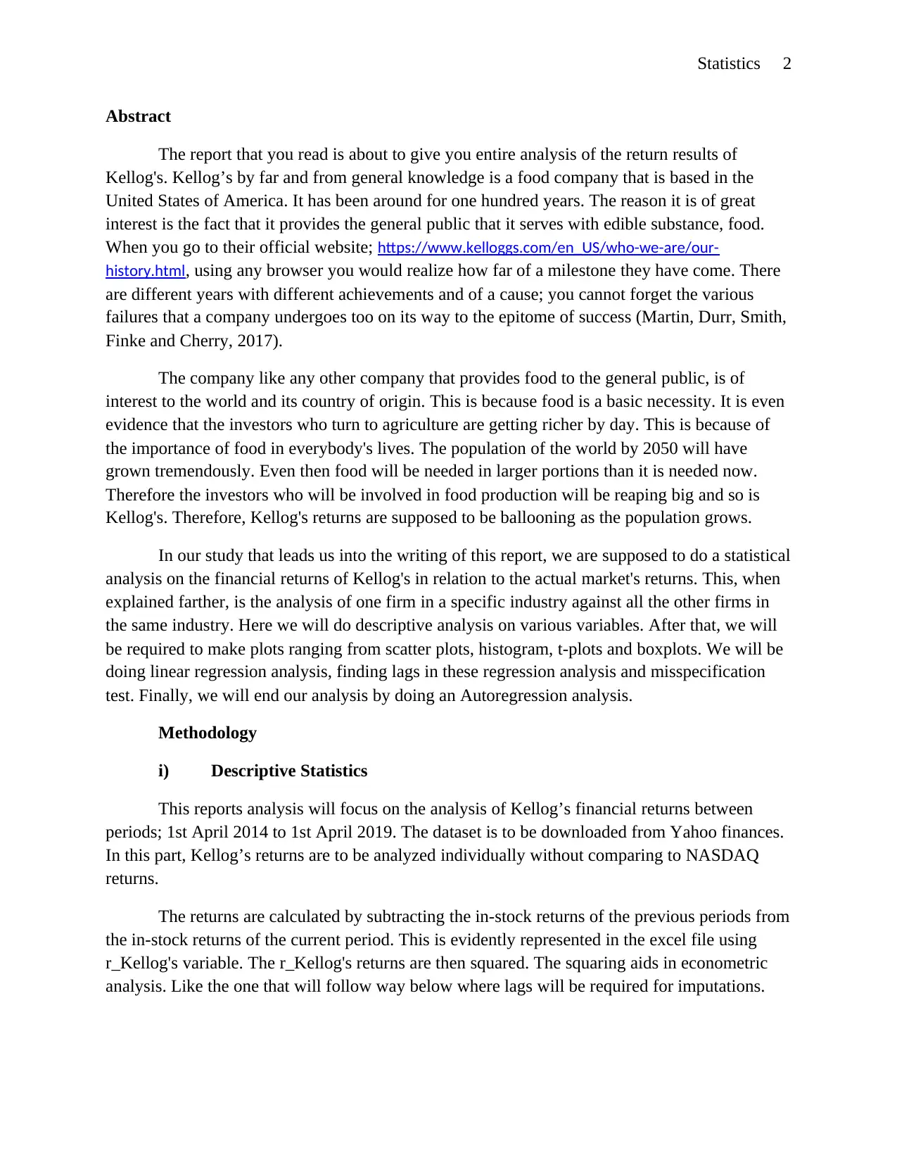
Figure 2
The descriptive statistics as per figure 2, on Kellog's absolute return, give a dataset with
mean and median very close in value. This indicates that the data is not so skewed from the
centre. The standard deviation value is less than the mean value, an indication that the variable
points are clustered just around the centre. The variance I the small, an indication that points are
not so far apart. The sum gives us a positive value.
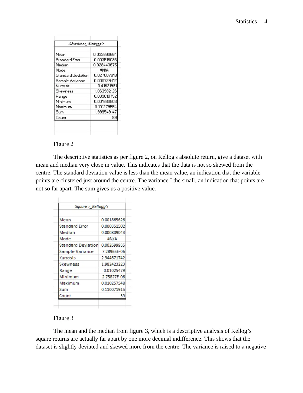
Figure 3
The mean and the median from figure 3, which is a descriptive analysis of Kellog’s
square returns are actually far apart by one more decimal indifference. This shows that the
dataset is slightly deviated and skewed more from the centre. The variance is raised to a negative
Figure 2
The descriptive statistics as per figure 2, on Kellog's absolute return, give a dataset with
mean and median very close in value. This indicates that the data is not so skewed from the
centre. The standard deviation value is less than the mean value, an indication that the variable
points are clustered just around the centre. The variance I the small, an indication that points are
not so far apart. The sum gives us a positive value.
Figure 3
The mean and the median from figure 3, which is a descriptive analysis of Kellog’s
square returns are actually far apart by one more decimal indifference. This shows that the
dataset is slightly deviated and skewed more from the centre. The variance is raised to a negative
Paraphrase This Document
Need a fresh take? Get an instant paraphrase of this document with our AI Paraphraser
Statistics 5
power; indicating the least distance between variables. The standard deviation which illustrates
how variables are well clustered to the centre actually serves a positive sign with all the variables
actually clustered a lot more at the centre. The sum is positive.
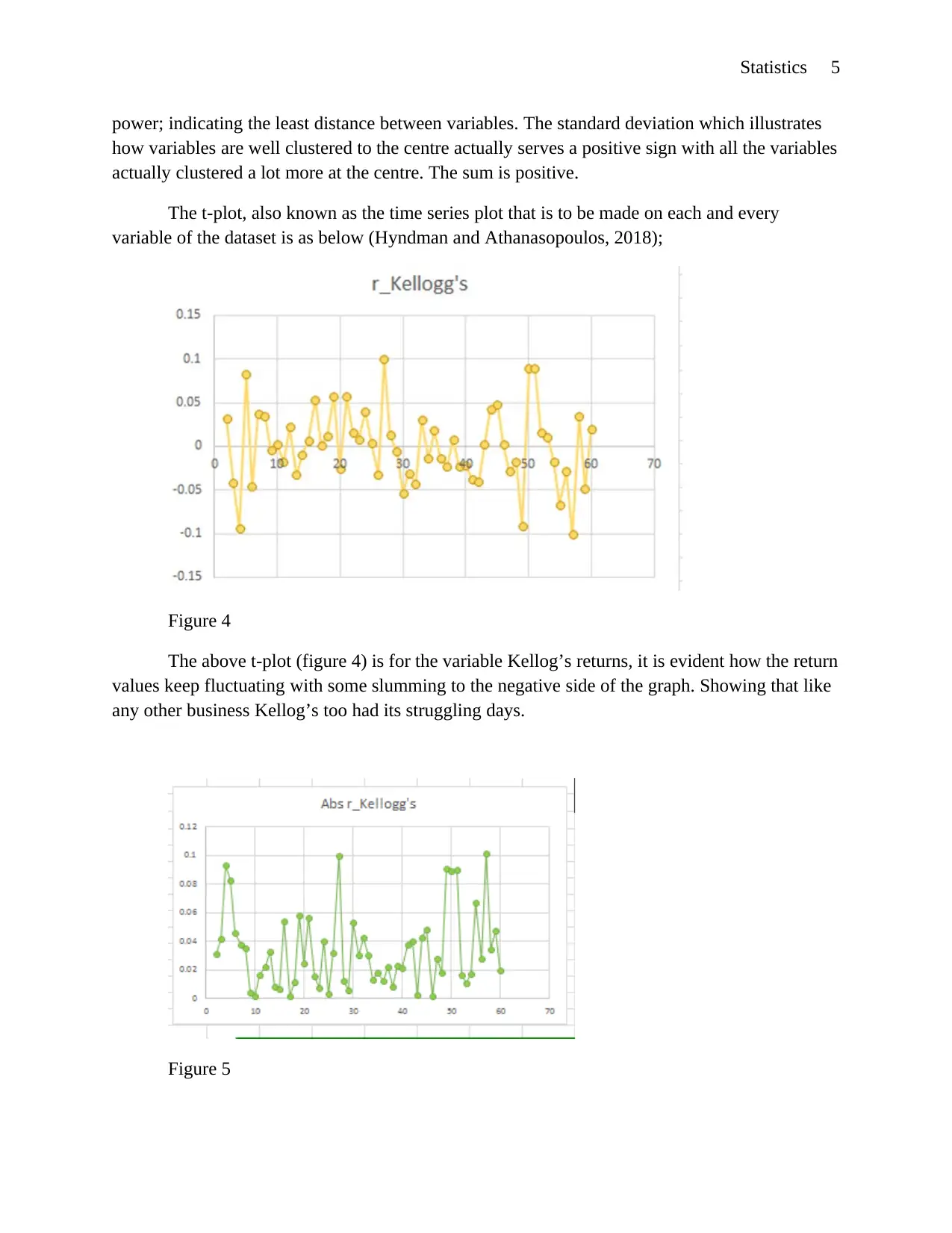
The t-plot, also known as the time series plot that is to be made on each and every
variable of the dataset is as below (Hyndman and Athanasopoulos, 2018);
Figure 4
The above t-plot (figure 4) is for the variable Kellog’s returns, it is evident how the return
values keep fluctuating with some slumming to the negative side of the graph. Showing that like
any other business Kellog’s too had its struggling days.
Figure 5
power; indicating the least distance between variables. The standard deviation which illustrates
how variables are well clustered to the centre actually serves a positive sign with all the variables
actually clustered a lot more at the centre. The sum is positive.
The t-plot, also known as the time series plot that is to be made on each and every
variable of the dataset is as below (Hyndman and Athanasopoulos, 2018);
Figure 4
The above t-plot (figure 4) is for the variable Kellog’s returns, it is evident how the return
values keep fluctuating with some slumming to the negative side of the graph. Showing that like
any other business Kellog’s too had its struggling days.
Figure 5
Statistics 6
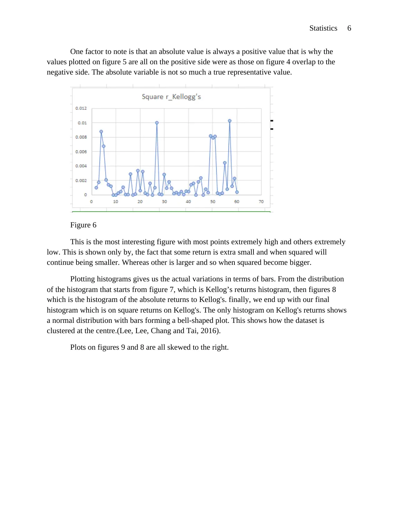
One factor to note is that an absolute value is always a positive value that is why the
values plotted on figure 5 are all on the positive side were as those on figure 4 overlap to the
negative side. The absolute variable is not so much a true representative value.
Figure 6
This is the most interesting figure with most points extremely high and others extremely
low. This is shown only by, the fact that some return is extra small and when squared will
continue being smaller. Whereas other is larger and so when squared become bigger.
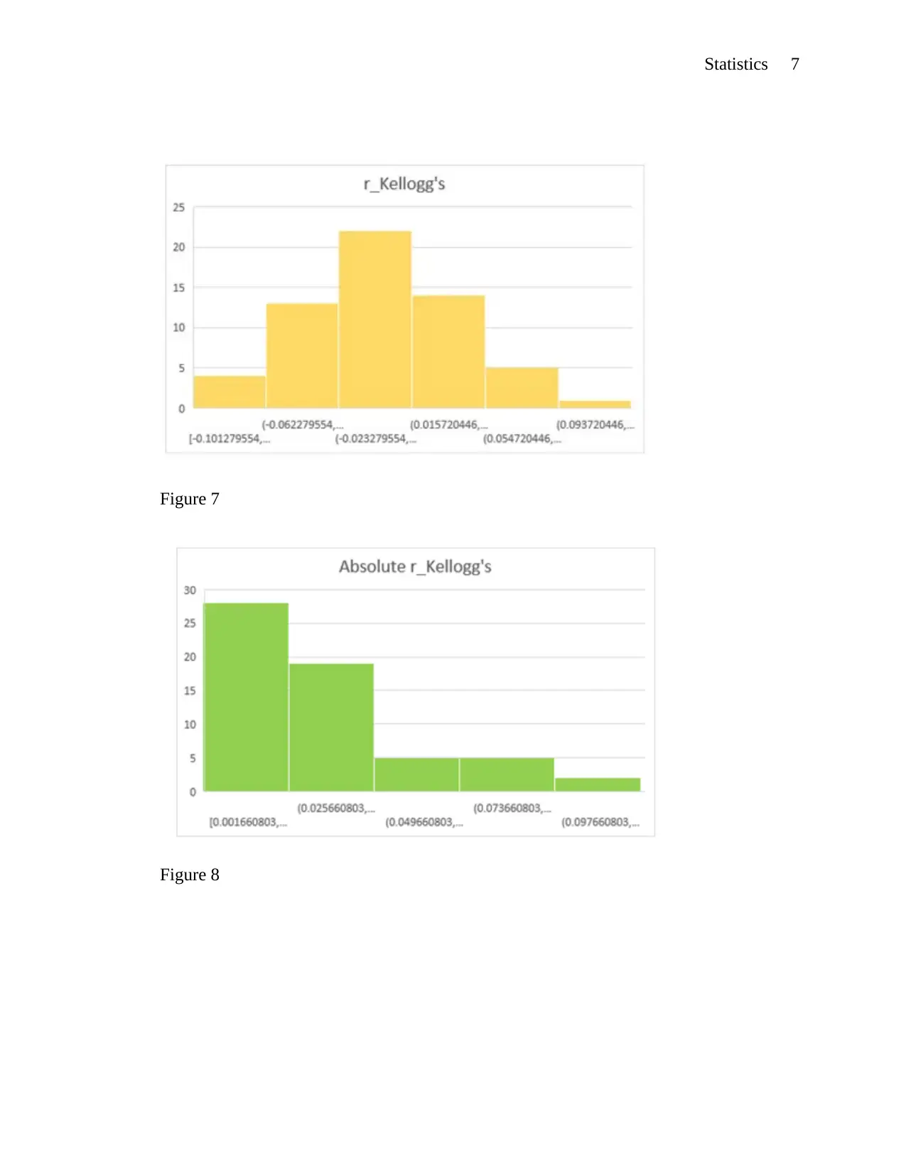
Plotting histograms gives us the actual variations in terms of bars. From the distribution
of the histogram that starts from figure 7, which is Kellog’s returns histogram, then figures 8
which is the histogram of the absolute returns to Kellog's. finally, we end up with our final
histogram which is on square returns on Kellog's. The only histogram on Kellog's returns shows
a normal distribution with bars forming a bell-shaped plot. This shows how the dataset is
clustered at the centre.(Lee, Lee, Chang and Tai, 2016).
Plots on figures 9 and 8 are all skewed to the right.
One factor to note is that an absolute value is always a positive value that is why the
values plotted on figure 5 are all on the positive side were as those on figure 4 overlap to the
negative side. The absolute variable is not so much a true representative value.
Figure 6
This is the most interesting figure with most points extremely high and others extremely
low. This is shown only by, the fact that some return is extra small and when squared will
continue being smaller. Whereas other is larger and so when squared become bigger.
Plotting histograms gives us the actual variations in terms of bars. From the distribution
of the histogram that starts from figure 7, which is Kellog’s returns histogram, then figures 8
which is the histogram of the absolute returns to Kellog's. finally, we end up with our final
histogram which is on square returns on Kellog's. The only histogram on Kellog's returns shows
a normal distribution with bars forming a bell-shaped plot. This shows how the dataset is
clustered at the centre.(Lee, Lee, Chang and Tai, 2016).
Plots on figures 9 and 8 are all skewed to the right.
⊘ This is a preview!⊘
Do you want full access?
Subscribe today to unlock all pages.
Trusted by 1+ million students worldwide
Statistics 7
Figure 7
Figure 8
Figure 7
Figure 8
Paraphrase This Document
Need a fresh take? Get an instant paraphrase of this document with our AI Paraphraser

Statistics 8
Figure 9
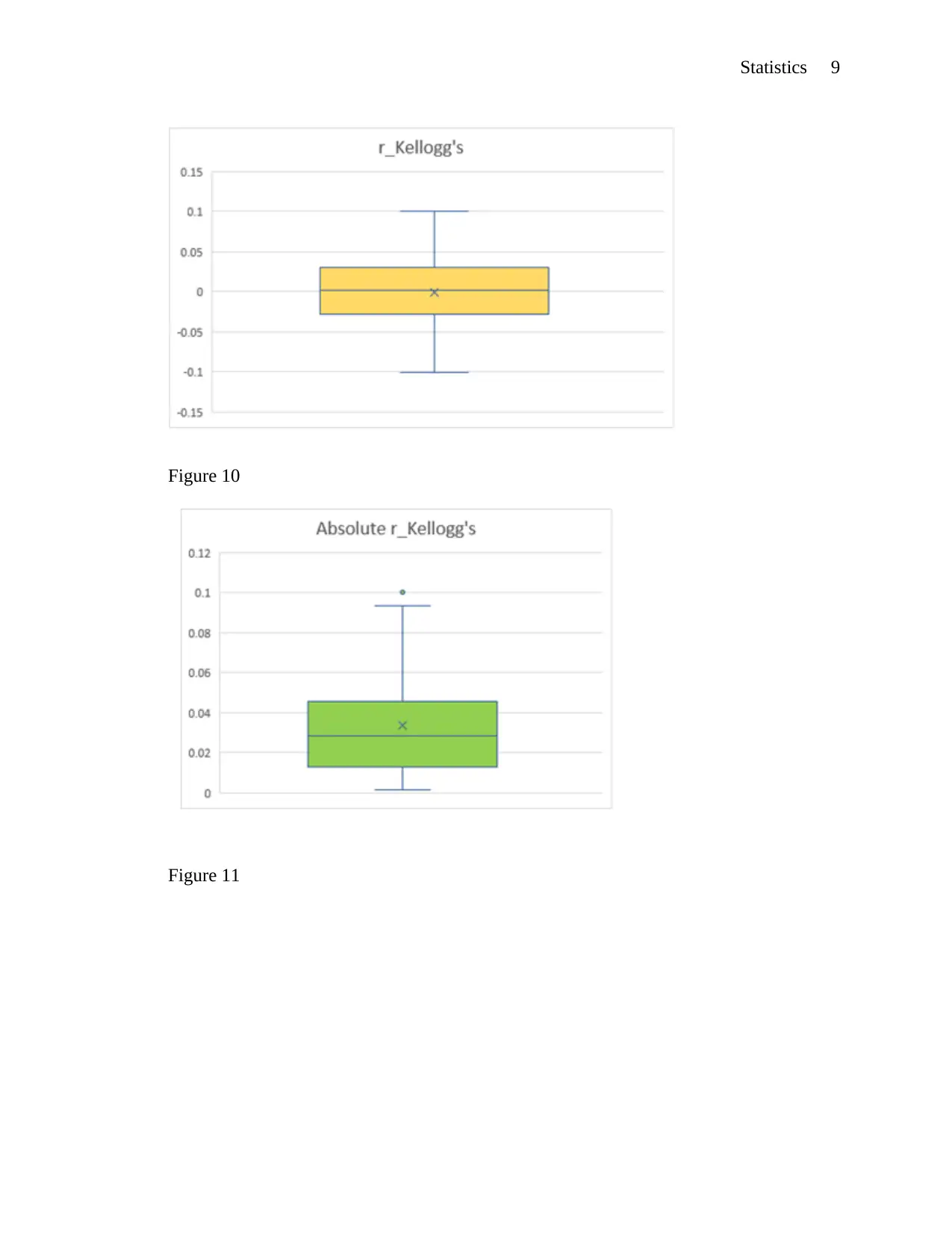
The very final plots that need to be made are the box and whiskers plots. This is a unique
plot and workload of plotting it depends on which version of excel you are specifically using. If
for instance you are using excels 2010 and below to make the plot, more workload will be
needed. If you are using excel 2013 and above then the workload will greatly reduce as most of
the steps of doing this are direct. The major idea of plotting box plots is to help check the
available outliers in a specific variable. Of all the respective boxplots that I have made, there are
outliers realized with the boxplot of absolute Kellog’s returns and more realized on the square
returns on Kellog’s. This is a true indication that the values of the variables that I am to use in
this analysis case are statistically less significant. The plotting of the boxplots will definitely
need, minimum, maximum and the quartile ranges for plots. Then the blots will be gotten from
the insert section, after which the version that you use will determine what way you will be
required to go (Carroll, 2016). An example of a boxplot is as below;
Figure 9
The very final plots that need to be made are the box and whiskers plots. This is a unique
plot and workload of plotting it depends on which version of excel you are specifically using. If
for instance you are using excels 2010 and below to make the plot, more workload will be
needed. If you are using excel 2013 and above then the workload will greatly reduce as most of
the steps of doing this are direct. The major idea of plotting box plots is to help check the
available outliers in a specific variable. Of all the respective boxplots that I have made, there are
outliers realized with the boxplot of absolute Kellog’s returns and more realized on the square
returns on Kellog’s. This is a true indication that the values of the variables that I am to use in
this analysis case are statistically less significant. The plotting of the boxplots will definitely
need, minimum, maximum and the quartile ranges for plots. Then the blots will be gotten from
the insert section, after which the version that you use will determine what way you will be
required to go (Carroll, 2016). An example of a boxplot is as below;
Statistics 9
Figure 10
Figure 11
Figure 10
Figure 11
⊘ This is a preview!⊘
Do you want full access?
Subscribe today to unlock all pages.
Trusted by 1+ million students worldwide
Statistics 10
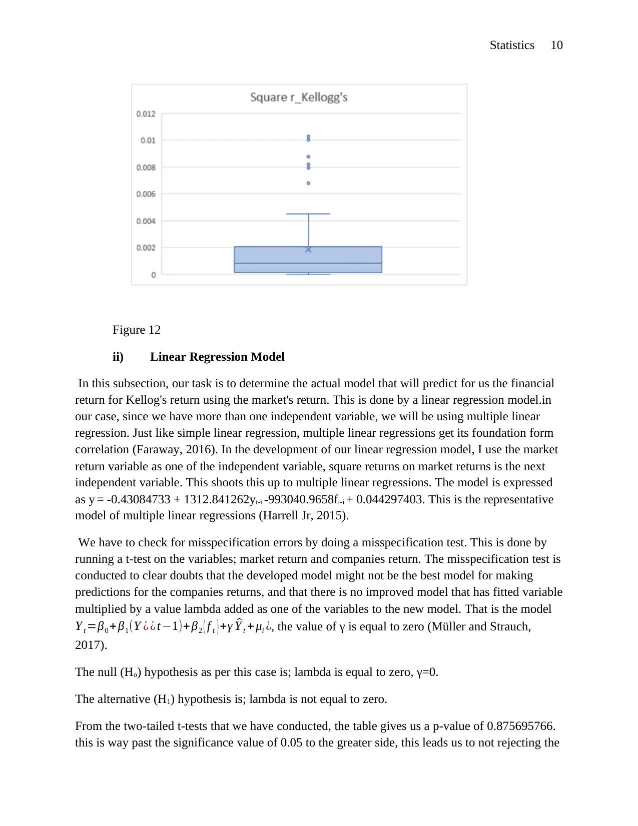
Figure 12
ii) Linear Regression Model
In this subsection, our task is to determine the actual model that will predict for us the financial
return for Kellog's return using the market's return. This is done by a linear regression model.in
our case, since we have more than one independent variable, we will be using multiple linear
regression. Just like simple linear regression, multiple linear regressions get its foundation form
correlation (Faraway, 2016). In the development of our linear regression model, I use the market
return variable as one of the independent variable, square returns on market returns is the next
independent variable. This shoots this up to multiple linear regressions. The model is expressed
as y = -0.43084733 + 1312.841262yt-i -993040.9658ft-i + 0.044297403. This is the representative
model of multiple linear regressions (Harrell Jr, 2015).
We have to check for misspecification errors by doing a misspecification test. This is done by
running a t-test on the variables; market return and companies return. The misspecification test is
conducted to clear doubts that the developed model might not be the best model for making
predictions for the companies returns, and that there is no improved model that has fitted variable
multiplied by a value lambda added as one of the variables to the new model. That is the model
Y t =β0 +β1(Y ¿ ¿ t −1)+ β2 ( f t ) +γ ^Y t + μi ¿, the value of γ is equal to zero (Müller and Strauch,
2017).
The null (Ho) hypothesis as per this case is; lambda is equal to zero, γ=0.
The alternative (H1) hypothesis is; lambda is not equal to zero.
From the two-tailed t-tests that we have conducted, the table gives us a p-value of 0.875695766.
this is way past the significance value of 0.05 to the greater side, this leads us to not rejecting the
Paraphrase This Document
Need a fresh take? Get an instant paraphrase of this document with our AI Paraphraser
Statistics 11
null hypothesis, and therefore there is no other better model as opposed to the model that we
have developed already (Quirk and Cummings, 2017).
The number of lags that sets the model to be more statistically adequate is 3. If we take
the company returns and develops a lag table with the company returns variable forming the y-
variables and the lags forming the x-variables. The regression results give an improvement to the
regression model with improved R values and improved p values.
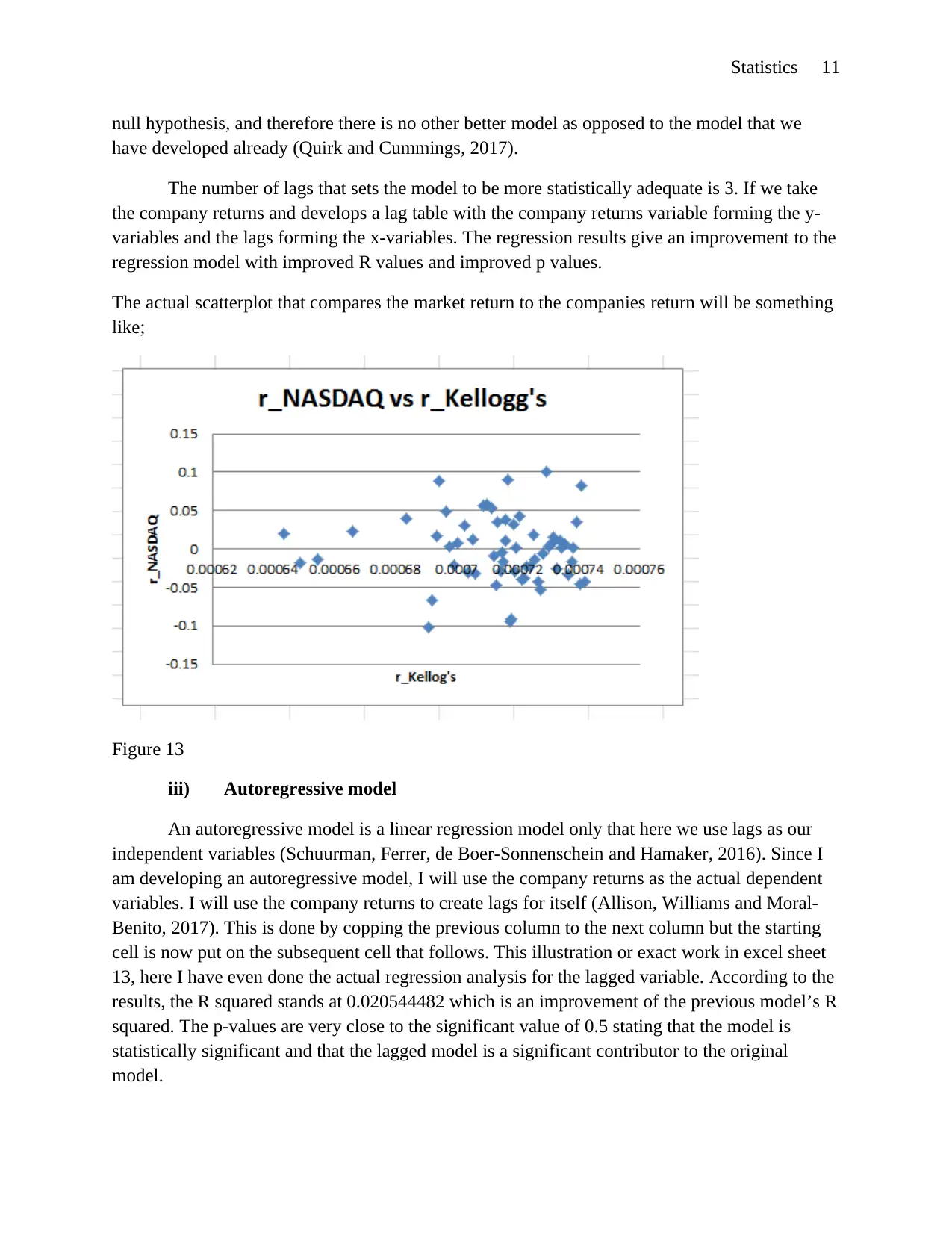
The actual scatterplot that compares the market return to the companies return will be something
like;
Figure 13
iii) Autoregressive model
An autoregressive model is a linear regression model only that here we use lags as our
independent variables (Schuurman, Ferrer, de Boer-Sonnenschein and Hamaker, 2016). Since I
am developing an autoregressive model, I will use the company returns as the actual dependent
variables. I will use the company returns to create lags for itself (Allison, Williams and Moral-
Benito, 2017). This is done by copping the previous column to the next column but the starting
cell is now put on the subsequent cell that follows. This illustration or exact work in excel sheet
13, here I have even done the actual regression analysis for the lagged variable. According to the
results, the R squared stands at 0.020544482 which is an improvement of the previous model’s R
squared. The p-values are very close to the significant value of 0.5 stating that the model is
statistically significant and that the lagged model is a significant contributor to the original
model.
null hypothesis, and therefore there is no other better model as opposed to the model that we
have developed already (Quirk and Cummings, 2017).
The number of lags that sets the model to be more statistically adequate is 3. If we take
the company returns and develops a lag table with the company returns variable forming the y-
variables and the lags forming the x-variables. The regression results give an improvement to the
regression model with improved R values and improved p values.
The actual scatterplot that compares the market return to the companies return will be something
like;
Figure 13
iii) Autoregressive model
An autoregressive model is a linear regression model only that here we use lags as our
independent variables (Schuurman, Ferrer, de Boer-Sonnenschein and Hamaker, 2016). Since I
am developing an autoregressive model, I will use the company returns as the actual dependent
variables. I will use the company returns to create lags for itself (Allison, Williams and Moral-
Benito, 2017). This is done by copping the previous column to the next column but the starting
cell is now put on the subsequent cell that follows. This illustration or exact work in excel sheet
13, here I have even done the actual regression analysis for the lagged variable. According to the
results, the R squared stands at 0.020544482 which is an improvement of the previous model’s R
squared. The p-values are very close to the significant value of 0.5 stating that the model is
statistically significant and that the lagged model is a significant contributor to the original
model.
Statistics 12
From the misspecification test, checking the F-test results and moving on to check the individual
values of the lag variables plus the t-test p-value results, we can be able to see that the actual
values are more than the significance value of 0.5. This leads us to pick the null hypothesis
which states that lambda is equal to zero and that there is no better model that can be picked to
serve the purpose of the model already developed for making predictions. Looking at the lagged
model developed we can the write a regression model out of it, the model therefore will look
like; y = 0.001657258 + -0.050043923N + 0.104205994N + -0.07002663N + 0.043050477.
Making projections for 5 years will give us a value of; 0.001657258 + -0.050043923(60) +
0.104205994(60) + -0.07002663(60) + 0.043050477 = -0.9071658.
The value of 60 is gotten after multiplying the number of years to the number of months in a
year, because the returns are computed monthly and therefore the returns too must be computed
monthly, hence the value realized. You must realize that the actual value is negative, not all
times does a business make profits, and there is a time that it must make a loss, hence the
negative value.
Conclusion
For the best models, it is better to use, the same variable to form its own lag variables.
There is a very strong correlation between autoregressive model and linear regression. The
autoregressive model uses lagged variables as the independent variables but the linear regression
uses other independent variables for regression. All in all, both the regression and the
autoregressive models are correlations. Lagged models produce improved models in most cases
with improved R squared and adjusted R squared values together with the values of the F
significance and the p-value. The t-test explains better how the actual misspecification error
occurs and how to test for lack of its existence by looking at the p-values. Excel too is a rich area
for econometrics.
⊘ This is a preview!⊘
Do you want full access?
Subscribe today to unlock all pages.
Trusted by 1+ million students worldwide
1 out of 13


Your All-in-One AI-Powered Toolkit for Academic Success.
+13062052269
info@desklib.com
Available 24*7 on WhatsApp / Email
![[object Object]](/_next/static/media/star-bottom.7253800d.svg)
Unlock your academic potential
Copyright © 2020–2026 A2Z Services. All Rights Reserved. Developed and managed by ZUCOL.