Business Report: House Price Appraisal in Melbourne Suburbs

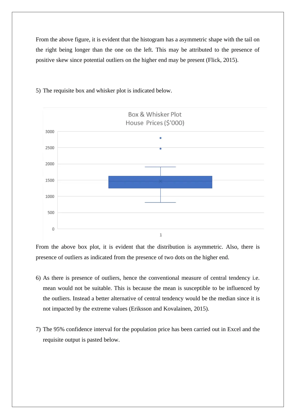
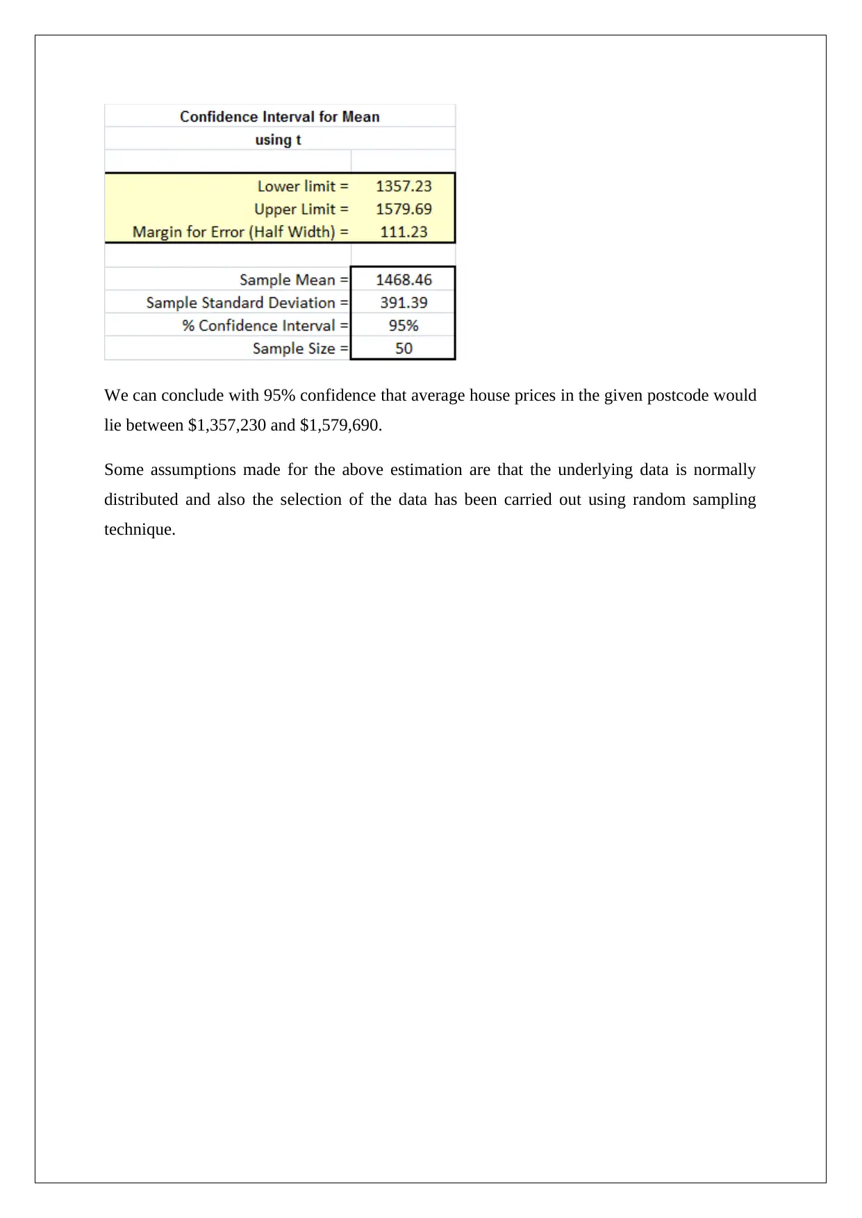
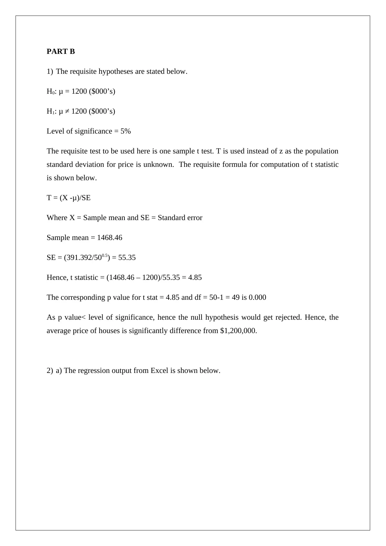
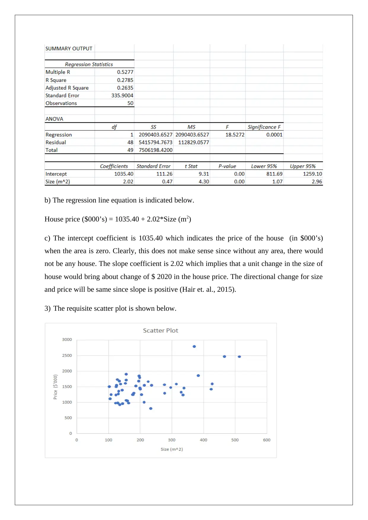
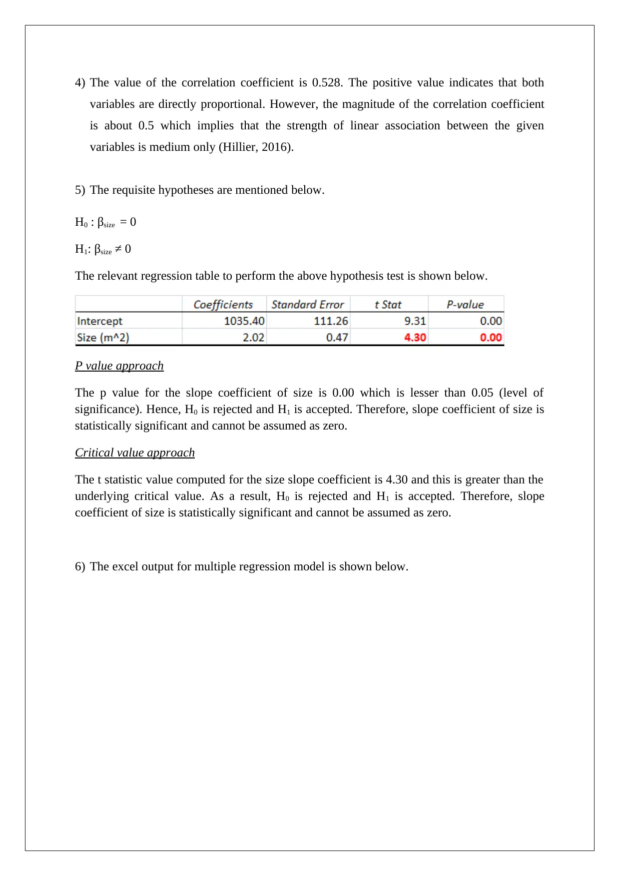
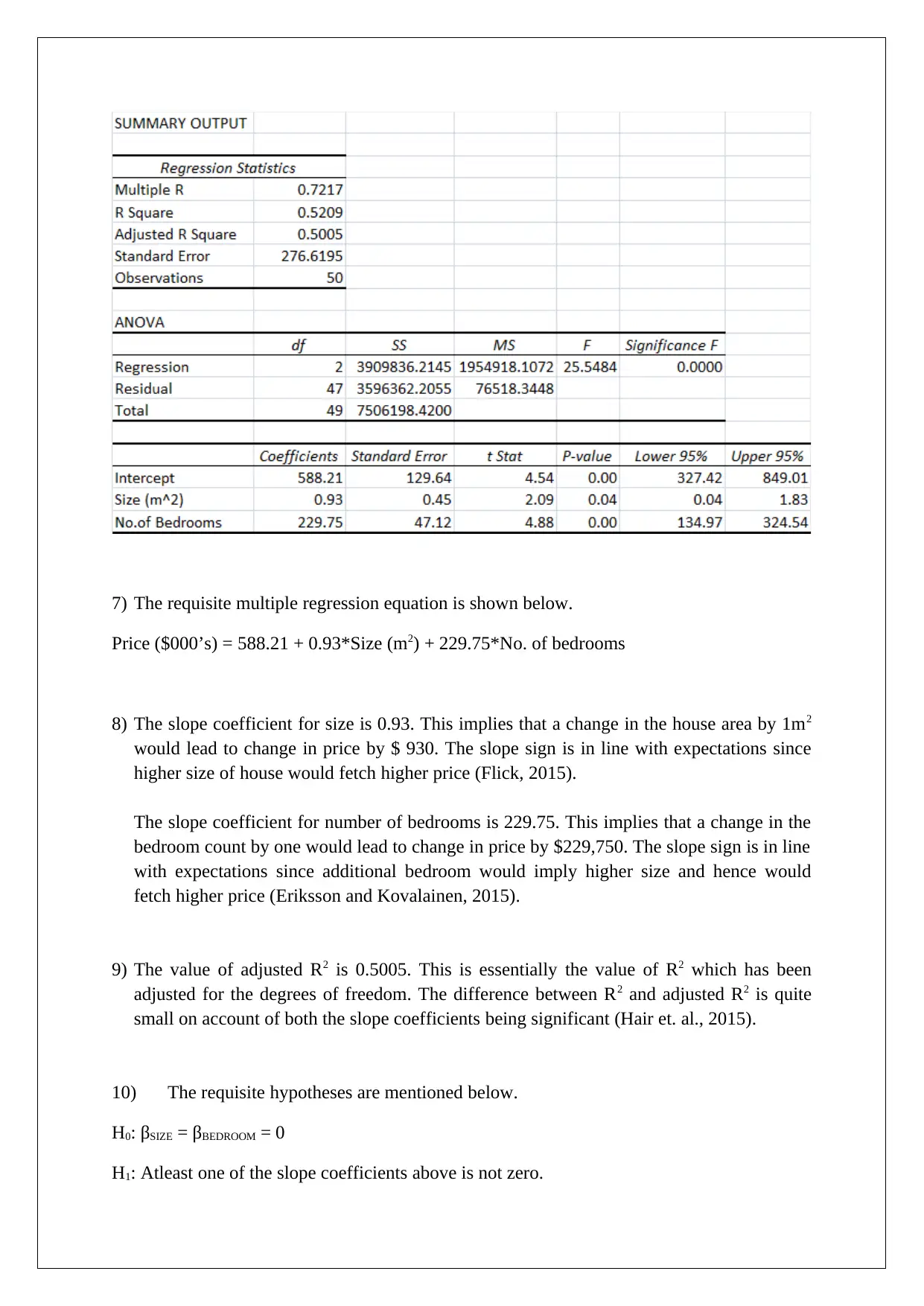
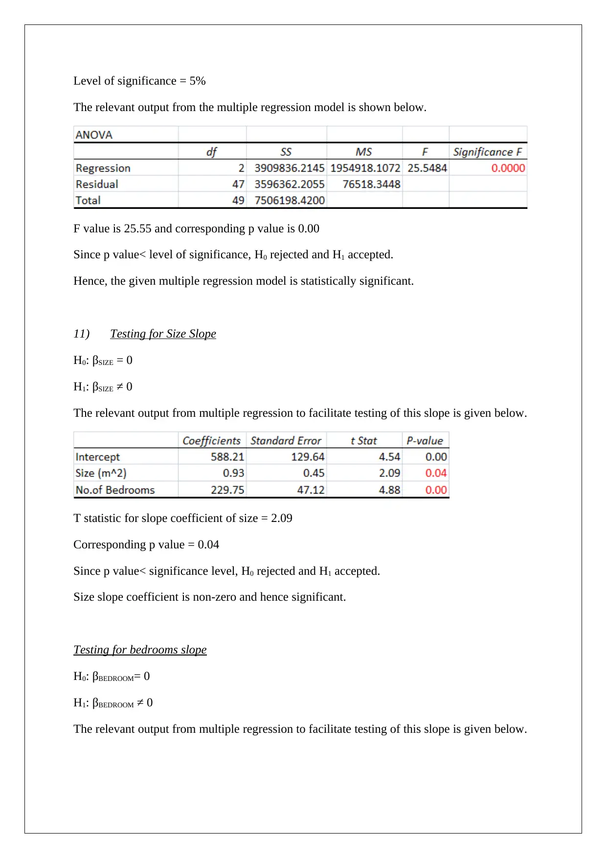
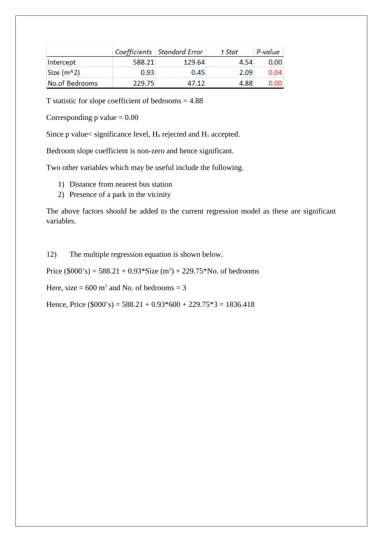
This report presents a statistical analysis of house prices in the Clifton Hill and Fitzroy North areas of Melbourne. It begins with descriptive statistics of key variables like price, size, and number of bedrooms, including their distributions and potential outliers. The analysis employs both simple and multiple linear regression models to estimate house prices, assessing the significance of various factors. The report includes hypothesis testing, confidence intervals, and the evaluation of regression coefficients. It explores model improvements and provides recommendations for enhancing predictive power. Furthermore, the report emphasizes the importance of presenting information in a manner accessible to a multilingual audience, including the use of visual aids and simplified representations of complex statistical results.

BUSINESS STATISTICS
STUDENT ID:
[Pick the date]

PART A
1) The requisite data as captured in the tabular format is shown below.

2) The Excel output with regards to descriptive statistics of the above variables is pasted
below.
3) The description for each of the variables is given below.
Price
The mean price of the sample is $1,468,460. This is different from the median price of $
1,460,000. This implies that the underlying variable is not normally distributed. Also, there is
a significant skew of 1.2 present which implies asymmetric shape whereby the tail on the
right of the mean is longer than the one on the left. The dispersion in this variable seems
medium considering the measures such as standard deviation, variance and range.
Size
The mean size of the sample is 214.88 m2. This is different from the median size of 183 m2.
This implies that the underlying variable is not normally distributed. Also, there is a
significant skew of 1.25 present which implies asymmetric shape whereby the tail on the
right of the mean is longer than the one on the left. The dispersion in this variable seems high
considering the measures such as standard deviation, variance and range.
Number of bedrooms
The mean number of bedrooms of the sample is 2.96. This is different from the median
bedroom count of 3. This implies that the underlying variable is not normally distributed.

Also, there is a significant skew of 1.35 present which implies asymmetric shape whereby the
tail on the right of the mean is longer than the one on the left. The dispersion in this variable
seems medium considering the measures such as standard deviation, variance and range.
4) The requisite histogram and frequency polygon has been indicated as follows.

From the above figure, it is evident that the histogram has a asymmetric shape with the tail on
the right being longer than the one on the left. This may be attributed to the presence of
positive skew since potential outliers on the higher end may be present (Flick, 2015).
5) The requisite box and whisker plot is indicated below.
From the above box plot, it is evident that the distribution is asymmetric. Also, there is
presence of outliers as indicated from the presence of two dots on the higher end.
6) As there is presence of outliers, hence the conventional measure of central tendency i.e.
mean would not be suitable. This is because the mean is susceptible to be influenced by
the outliers. Instead a better alternative of central tendency would be the median since it is
not impacted by the extreme values (Eriksson and Kovalainen, 2015).
7) The 95% confidence interval for the population price has been carried out in Excel and the
requisite output is pasted below.

We can conclude with 95% confidence that average house prices in the given postcode would
lie between $1,357,230 and $1,579,690.
Some assumptions made for the above estimation are that the underlying data is normally
distributed and also the selection of the data has been carried out using random sampling
technique.

PART B
1) The requisite hypotheses are stated below.
H0: μ = 1200 ($000’s)
H1: μ ≠ 1200 ($000’s)
Level of significance = 5%
The requisite test to be used here is one sample t test. T is used instead of z as the population
standard deviation for price is unknown. The requisite formula for computation of t statistic
is shown below.
T = (X -μ)/SE
Where X = Sample mean and SE = Standard error
Sample mean = 1468.46
SE = (391.392/500.5) = 55.35
Hence, t statistic = (1468.46 – 1200)/55.35 = 4.85
The corresponding p value for t stat = 4.85 and df = 50-1 = 49 is 0.000
As p value< level of significance, hence the null hypothesis would get rejected. Hence, the
average price of houses is significantly difference from $1,200,000.
2) a) The regression output from Excel is shown below.

b) The regression line equation is indicated below.
House price ($000’s) = 1035.40 + 2.02*Size (m2)
c) The intercept coefficient is 1035.40 which indicates the price of the house (in $000’s)
when the area is zero. Clearly, this does not make sense since without any area, there would
not be any house. The slope coefficient is 2.02 which implies that a unit change in the size of
house would bring about change of $ 2020 in the house price. The directional change for size
and price will be same since slope is positive (Hair et. al., 2015).
3) The requisite scatter plot is shown below.

4) The value of the correlation coefficient is 0.528. The positive value indicates that both
variables are directly proportional. However, the magnitude of the correlation coefficient
is about 0.5 which implies that the strength of linear association between the given
variables is medium only (Hillier, 2016).
5) The requisite hypotheses are mentioned below.
H0 : βsize = 0
H1: βsize ≠ 0
The relevant regression table to perform the above hypothesis test is shown below.
P value approach
The p value for the slope coefficient of size is 0.00 which is lesser than 0.05 (level of
significance). Hence, H0 is rejected and H1 is accepted. Therefore, slope coefficient of size is
statistically significant and cannot be assumed as zero.
Critical value approach
The t statistic value computed for the size slope coefficient is 4.30 and this is greater than the
underlying critical value. As a result, H0 is rejected and H1 is accepted. Therefore, slope
coefficient of size is statistically significant and cannot be assumed as zero.
6) The excel output for multiple regression model is shown below.

7) The requisite multiple regression equation is shown below.
Price ($000’s) = 588.21 + 0.93*Size (m2) + 229.75*No. of bedrooms
8) The slope coefficient for size is 0.93. This implies that a change in the house area by 1m2
would lead to change in price by $ 930. The slope sign is in line with expectations since
higher size of house would fetch higher price (Flick, 2015).
The slope coefficient for number of bedrooms is 229.75. This implies that a change in the
bedroom count by one would lead to change in price by $229,750. The slope sign is in line
with expectations since additional bedroom would imply higher size and hence would
fetch higher price (Eriksson and Kovalainen, 2015).
9) The value of adjusted R2 is 0.5005. This is essentially the value of R2 which has been
adjusted for the degrees of freedom. The difference between R2 and adjusted R2 is quite
small on account of both the slope coefficients being significant (Hair et. al., 2015).
10) The requisite hypotheses are mentioned below.
H0: βSIZE = βBEDROOM = 0
H1: Atleast one of the slope coefficients above is not zero.

Level of significance = 5%
The relevant output from the multiple regression model is shown below.
F value is 25.55 and corresponding p value is 0.00
Since p value< level of significance, H0 rejected and H1 accepted.
Hence, the given multiple regression model is statistically significant.
11) Testing for Size Slope
H0: βSIZE = 0
H1: βSIZE ≠ 0
The relevant output from multiple regression to facilitate testing of this slope is given below.
T statistic for slope coefficient of size = 2.09
Corresponding p value = 0.04
Since p value< significance level, H0 rejected and H1 accepted.
Size slope coefficient is non-zero and hence significant.
Testing for bedrooms slope
H0: βBEDROOM= 0
H1: βBEDROOM ≠ 0
The relevant output from multiple regression to facilitate testing of this slope is given below.

T statistic for slope coefficient of bedrooms = 4.88
Corresponding p value = 0.00
Since p value< significance level, H0 rejected and H1 accepted.
Bedroom slope coefficient is non-zero and hence significant.
Two other variables which may be useful include the following.
1) Distance from nearest bus station
2) Presence of a park in the vicinity
The above factors should be added to the current regression model as these are significant
variables.
12) The multiple regression equation is shown below.
Price ($000’s) = 588.21 + 0.93*Size (m2) + 229.75*No. of bedrooms
Here, size = 600 m2 and No. of bedrooms = 3
Hence, Price ($000’s) = 588.21 + 0.93*600 + 229.75*3 = 1836.418