Applied Statistical Methods: Data Analysis and Interpretation

This assignment focuses on applied statistical methods, utilizing a provided dataset to analyze a continuous quantitative variable, "z7". The solution develops descriptive statistics, frequency tables, and histograms for the entire dataset and for three subgroups created by dividing the data. The analysis includes measures of central tendency (mean, median, mode), variation (standard deviation, variance), and skewness. The assignment identifies the shape of the distribution for each group, contrasts the groups based on their statistical properties and visual representations (histograms), and explains the causes of the observed differences in skewness, referencing the position of data values relative to measures of central tendency. The document also includes an introduction, results, and references to support the analysis.

Running head: APPLIED STATISTICAL METHODS 1
Applied Statistical Methods
Student Name
Professor’s Name
University Name
Date

APPLIED STATISTICAL METHODS 2
Solution
Introduction
Data is provided and we need to identify a continuous quantitative variable. The variable
identified is “z7” since it’s the only continuous quantitative variable available in the dataset and
is used to develop descriptive statistics, frequency table with appropriate intervals and a
histogram. Additionally, the data is to be subdivided into sample for which descriptive statistics,
frequency table and histogram will be developed. We will report on the shape of distribution for
each, contrast the groups and explain the causes of the differences.
Results
Z7 Variable
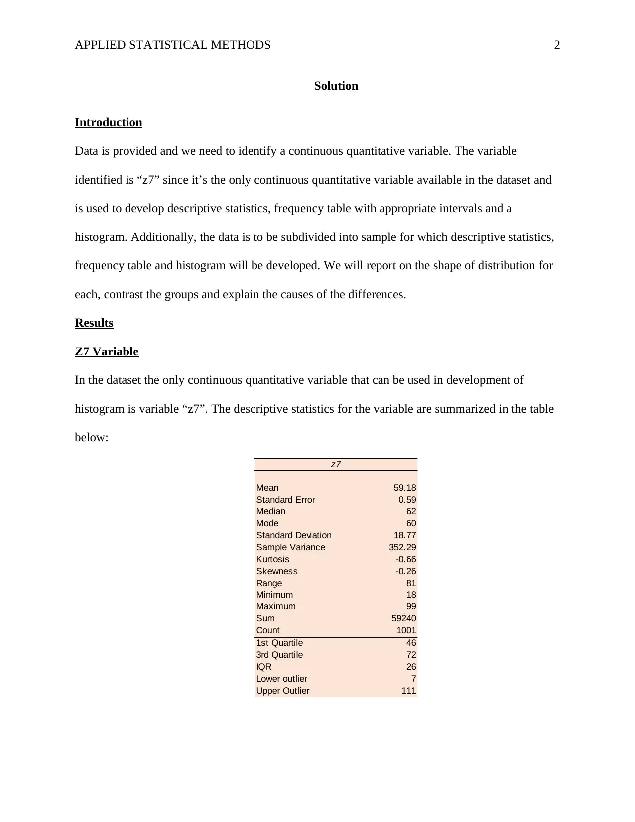
In the dataset the only continuous quantitative variable that can be used in development of
histogram is variable “z7”. The descriptive statistics for the variable are summarized in the table
below:
z7
Mean 59.18
Standard Error 0.59
Median 62
Mode 60
Standard Deviation 18.77
Sample Variance 352.29
Kurtosis -0.66
Skewness -0.26
Range 81
Minimum 18
Maximum 99
Sum 59240
Count 1001
1st Quartile 46
3rd Quartile 72
IQR 26
Lower outlier 7
Upper Outlier 111

APPLIED STATISTICAL METHODS 3
The measure of the central tendency or center are mean, median and mode while the measures of
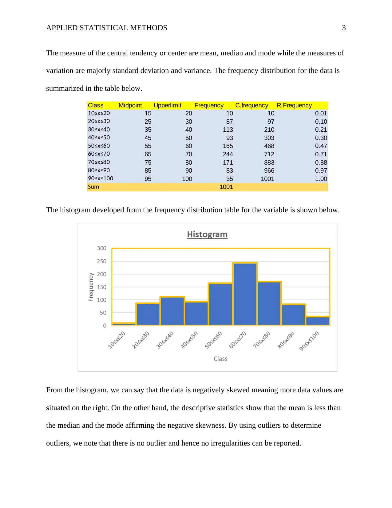
variation are majorly standard deviation and variance. The frequency distribution for the data is
summarized in the table below.
Class Midpoint Upperlimit Frequency C.frequency R.Frequency
10≤x≤20 15 20 10 10 0.01
20≤x≤30 25 30 87 97 0.10
30≤x≤40 35 40 113 210 0.21
40≤x≤50 45 50 93 303 0.30
50≤x≤60 55 60 165 468 0.47
60≤x≤70 65 70 244 712 0.71
70≤x≤80 75 80 171 883 0.88
80≤x≤90 85 90 83 966 0.97
90≤x≤100 95 100 35 1001 1.00
Sum 1001
The histogram developed from the frequency distribution table for the variable is shown below.
From the histogram, we can say that the data is negatively skewed meaning more data values are
situated on the right. On the other hand, the descriptive statistics show that the mean is less than
the median and the mode affirming the negative skewness. By using outliers to determine
outliers, we note that there is no outlier and hence no irregularities can be reported.

APPLIED STATISTICAL METHODS 4
Subgroups
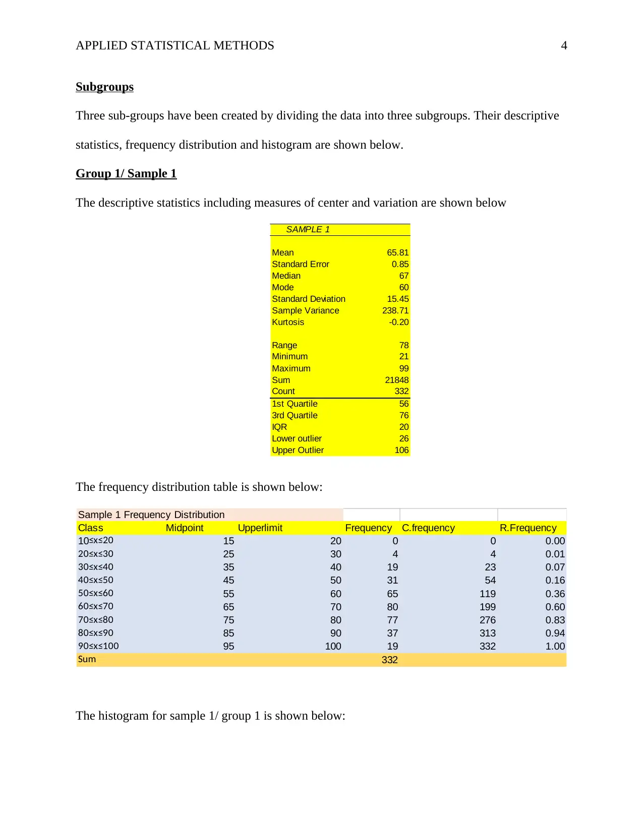
Three sub-groups have been created by dividing the data into three subgroups. Their descriptive
statistics, frequency distribution and histogram are shown below.
Group 1/ Sample 1
The descriptive statistics including measures of center and variation are shown below
SAMPLE 1
Mean 65.81
Standard Error 0.85
Median 67
Mode 60
Standard Deviation 15.45
Sample Variance 238.71
Kurtosis -0.20
Range 78
Minimum 21
Maximum 99
Sum 21848
Count 332
1st Quartile 56
3rd Quartile 76
IQR 20
Lower outlier 26
Upper Outlier 106
The frequency distribution table is shown below:
Sample 1 Frequency Distribution
Class Midpoint Upperlimit Frequency C.frequency R.Frequency
10≤x≤20 15 20 0 0 0.00
20≤x≤30 25 30 4 4 0.01
30≤x≤40 35 40 19 23 0.07
40≤x≤50 45 50 31 54 0.16
50≤x≤60 55 60 65 119 0.36
60≤x≤70 65 70 80 199 0.60
70≤x≤80 75 80 77 276 0.83
80≤x≤90 85 90 37 313 0.94
90≤x≤100 95 100 19 332 1.00
Sum 332
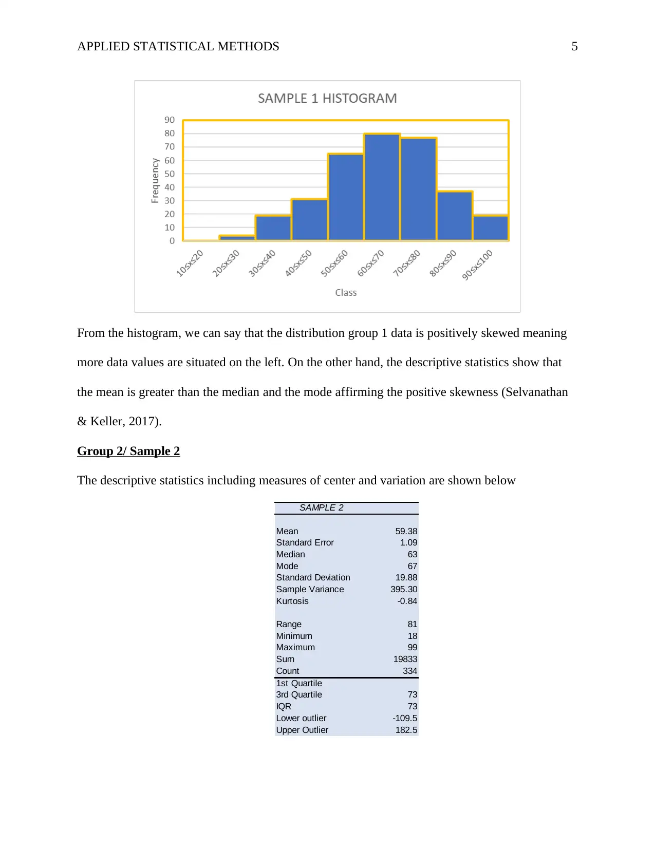
The histogram for sample 1/ group 1 is shown below:

APPLIED STATISTICAL METHODS 5
From the histogram, we can say that the distribution group 1 data is positively skewed meaning
more data values are situated on the left. On the other hand, the descriptive statistics show that
the mean is greater than the median and the mode affirming the positive skewness (Selvanathan
& Keller, 2017).
Group 2/ Sample 2
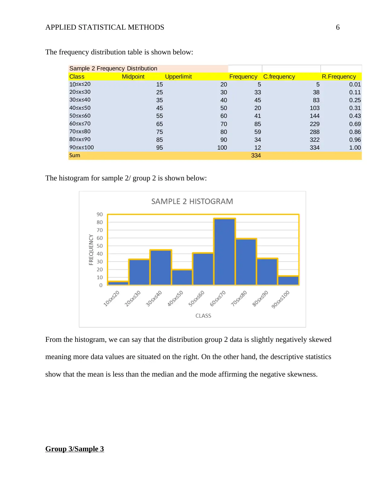
The descriptive statistics including measures of center and variation are shown below
SAMPLE 2
Mean 59.38
Standard Error 1.09
Median 63
Mode 67
Standard Deviation 19.88
Sample Variance 395.30
Kurtosis -0.84
Range 81
Minimum 18
Maximum 99
Sum 19833
Count 334
1st Quartile
3rd Quartile 73
IQR 73
Lower outlier -109.5
Upper Outlier 182.5

APPLIED STATISTICAL METHODS 6
The frequency distribution table is shown below:
Sample 2 Frequency Distribution
Class Midpoint Upperlimit Frequency C.frequency R.Frequency
10≤x≤20 15 20 5 5 0.01
20≤x≤30 25 30 33 38 0.11
30≤x≤40 35 40 45 83 0.25
40≤x≤50 45 50 20 103 0.31
50≤x≤60 55 60 41 144 0.43
60≤x≤70 65 70 85 229 0.69
70≤x≤80 75 80 59 288 0.86
80≤x≤90 85 90 34 322 0.96
90≤x≤100 95 100 12 334 1.00
Sum 334
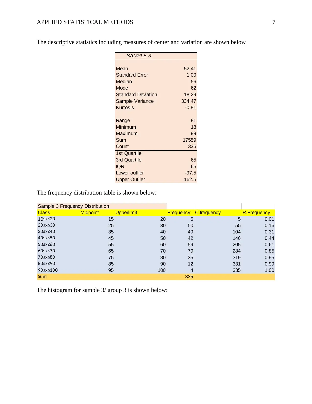
The histogram for sample 2/ group 2 is shown below:
From the histogram, we can say that the distribution group 2 data is slightly negatively skewed
meaning more data values are situated on the right. On the other hand, the descriptive statistics
show that the mean is less than the median and the mode affirming the negative skewness.
Group 3/Sample 3

APPLIED STATISTICAL METHODS 7
The descriptive statistics including measures of center and variation are shown below
SAMPLE 3
Mean 52.41
Standard Error 1.00
Median 56
Mode 62
Standard Deviation 18.29
Sample Variance 334.47
Kurtosis -0.81
Range 81
Minimum 18
Maximum 99
Sum 17559
Count 335
1st Quartile
3rd Quartile 65
IQR 65
Lower outlier -97.5
Upper Outlier 162.5
The frequency distribution table is shown below:
Sample 3 Frequency Distribution
Class Midpoint Upperlimit Frequency C.frequency R.Frequency
10≤x≤20 15 20 5 5 0.01
20≤x≤30 25 30 50 55 0.16
30≤x≤40 35 40 49 104 0.31
40≤x≤50 45 50 42 146 0.44
50≤x≤60 55 60 59 205 0.61
60≤x≤70 65 70 79 284 0.85
70≤x≤80 75 80 35 319 0.95
80≤x≤90 85 90 12 331 0.99
90≤x≤100 95 100 4 335 1.00
Sum 335
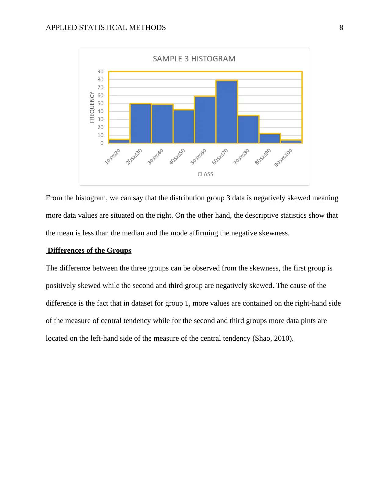
The histogram for sample 3/ group 3 is shown below:

APPLIED STATISTICAL METHODS 8
From the histogram, we can say that the distribution group 3 data is negatively skewed meaning
more data values are situated on the right. On the other hand, the descriptive statistics show that
the mean is less than the median and the mode affirming the negative skewness.
Differences of the Groups
The difference between the three groups can be observed from the skewness, the first group is
positively skewed while the second and third group are negatively skewed. The cause of the
difference is the fact that in dataset for group 1, more values are contained on the right-hand side
of the measure of central tendency while for the second and third groups more data pints are
located on the left-hand side of the measure of the central tendency (Shao, 2010).

APPLIED STATISTICAL METHODS 9
References
Selvanathan, E. A., & Keller, G. (2017). Business statistics abridged (7th ed). South
Melbourne, Victoria: Cengage Learning.
Shao, J. (2010). Mathematical statistics (2nd ed). New York: Springer.