University Epidemiology Assignment: Statistical Methods Explained

This assignment delves into various statistical methods crucial for epidemiology. It begins by explaining histograms and their applications, followed by the use of paired t-tests and independent t-tests. The assignment then explores confidence intervals and the coefficient of variation. It differentiates between confounding and effect modification, providing examples and explaining their roles in observational and randomized studies. The solution also covers confounding bias, stratification, and the rare disease assumption. Finally, it analyzes a case study involving cancer, sex, and smoking, calculating and interpreting odds ratios to determine effect modification and the influence of confounding variables like age. The assignment provides detailed explanations and calculations, making it a valuable resource for students studying epidemiology.

Running Head: STATISTICAL METHODS IN EPIDEMIOLOGY
Statistical Methods in Epidemiology
Name of the Student:
Name of the University:
Author Note:

1
STATISTICAL METHODS IN EPIDEMIOLOGY
Table of Contents
Answer to the question no. 1......................................................................................................2
Answer to the question no. 2......................................................................................................4
Answer to the question no. 3......................................................................................................5
References..................................................................................................................................8

2
STATISTICAL METHODS IN EPIDEMIOLOGY
Answer to the question no. 1
( )ⅰ Histogram is a graphical method which shows the frequency distribution a
continuous variable, which is introduced by Karl Pearson. It is define with the help of some
bar but there is no gap between the bar or rectangles. It is used to show frequency
distribution. It is also shows a rough sense of the density function. The area of histogram
define probability density which is 1. In some cases a histogram is used as a simplistic kernel
density function. Which gives more accurate distribution of the variable. It is represented
alternative to the histogram that means it is represented by some set of boxes. But the
correlate variation of a kernel density is difficult to represent, while it is simple in histogram
in case of frequency distribution.
(ⅱ) Given that a study involving a random sample of 36 sets of twin infants. One
member of each twin-pair is randomly chosen to receive diet A and the other diet B. The
one¬ month weight gain is measured for all 36x2=72 infants. In this case we wish to use
paired t-test. Because here there are two samples namely diet A and diet B and they are
related with equal size. Since the above the satisfied the above condition of paired t-test, so
this one is the appropriate test for the above data.
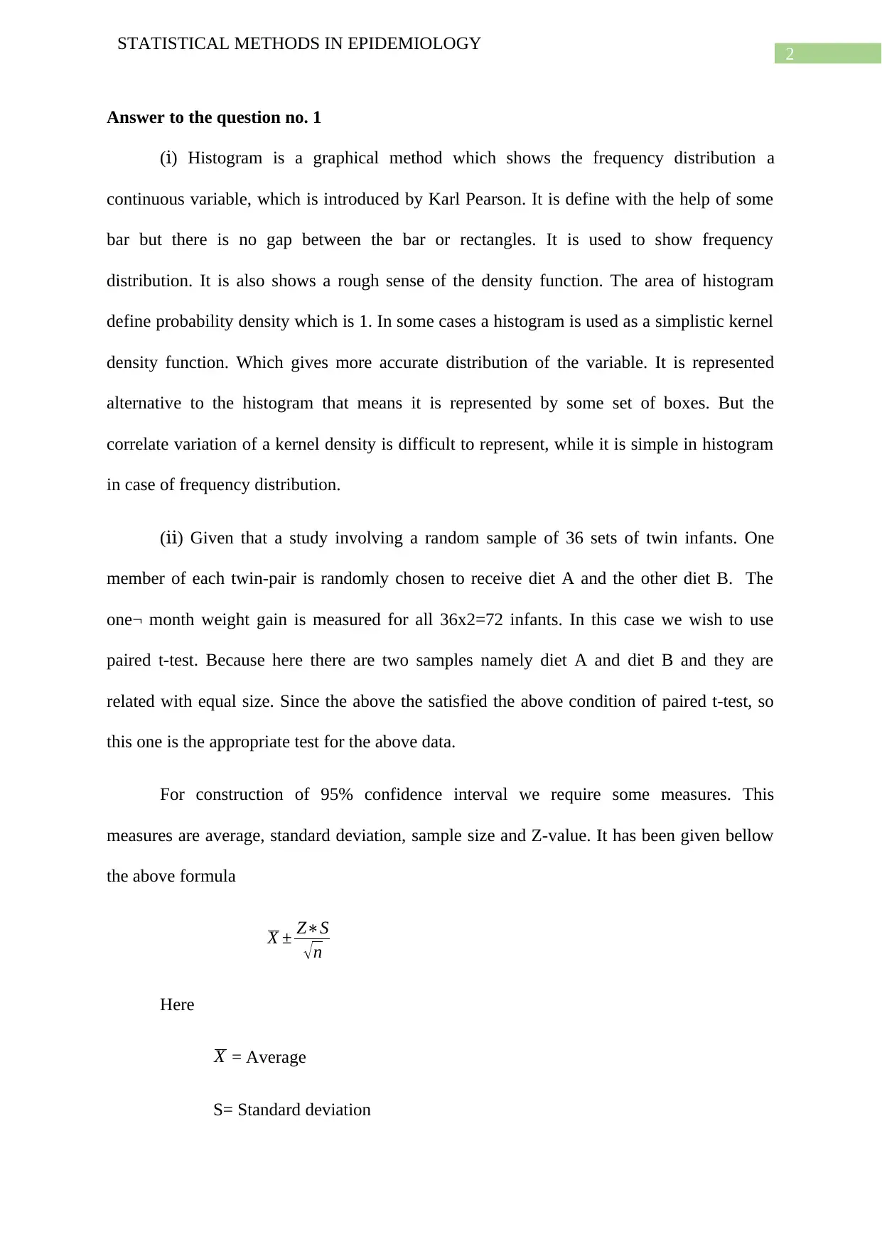
For construction of 95% confidence interval we require some measures. This
measures are average, standard deviation, sample size and Z-value. It has been given bellow
the above formula
X ± Z∗S
√ n
Here
X = Average
S= Standard deviation

3
STATISTICAL METHODS IN EPIDEMIOLOGY
n = Sample size
Z= Z-value (in this case at 95%)
First of all it has to calculate the difference between the two groups. Then it calculate
the average and standard deviation of the difference. From the above data it already have the
total sample size. For 95% the Z-value is (-1.96, 1.96). Putting all this value we get 95%
confidence interval.
( ) If the data is not correlated or paired then unequal variance independent t-test isⅲ
used. It use unequal variance independent t-test when the two sample sets have the same size
and unequal variance. In the above case it has been using this test because this data satisfied
all the condition which is required to use this test.
(ⅳ) When it has been compared the spread/variation for two variables with different
measurement scales, then it use coefficient of variation as a statistical measure. Because
when it calculate the variation for different measures then the coefficient variation is the only
and appropriate measure. To find coefficient of variation it require standard deviation and
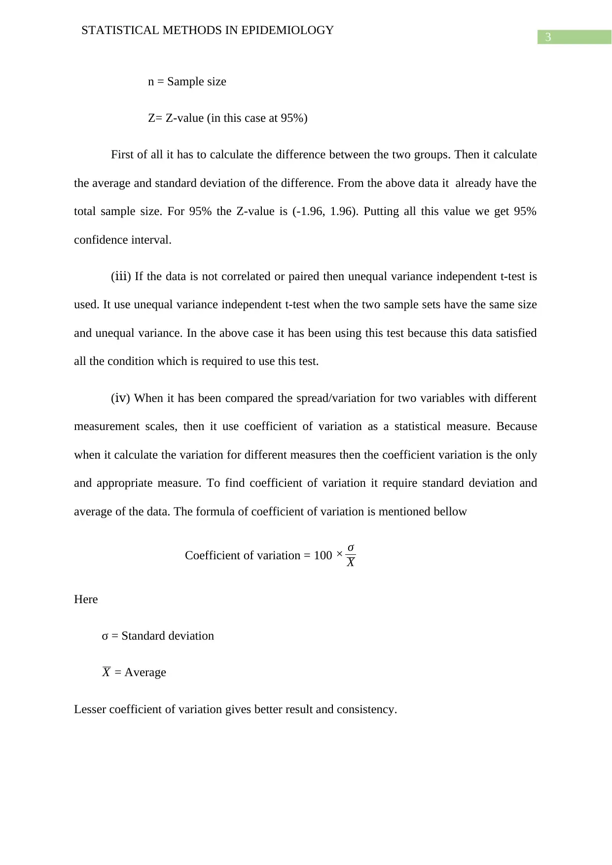
average of the data. The formula of coefficient of variation is mentioned bellow
Coefficient of variation = 100 × σ
X
Here
σ = Standard deviation
X = Average
Lesser coefficient of variation gives better result and consistency.

4
STATISTICAL METHODS IN EPIDEMIOLOGY
Answer to the question no. 2
(ⅰ) Confounding is a statistical measure which is commonly occurs in observational
studies and randomised studies. It influences both exposure and outcome. It is also defined as
a data generating model. Let us take an example, X denote the effectiveness of drug, Z denote
gender which influences to drug and Y denote recovery. In this case Z cofounds the
relationship between X and Y. From the above example it learn that confounding is a way
where it has seen that the effect of two variable is destroyed by the presence of another
variable.
Effect modification is a statistical modification way where it has modified the effect
positively and negatively. It is a factor where it effect only outcomes. It occurs when the
association between two depending on third variable. In effect modification we examine
effect separately for third variable.
Confounding effect is stronger than Effect modification. Because confounding is a
factor which is associated between exposure and outcome.
(ⅱ) Confounding is a way where we associate between exposure and outcome. Which
is distributed unequally. (Fleiss, Levin & Paik, 2013). In the presence of some
consequence in the disease exposure relationship we have some problem. In the
hypothetical cohort study while it test the association between exercise and heart
disease then age is the confounder. Because it is the risk factor for this disease. For
some people it is also prevent factor because exercise is good for health. There are
many factor for looking the association like age, diet and smoking.
Confounding bias is a type of error which is occur in epidemiologic studies.
(Lawson, 2013). Residual confounding is a confounding which occurs when the
confounder has not adjusted for the study. For example in a large age group.

5
STATISTICAL METHODS IN EPIDEMIOLOGY
(ⅲ) Confounding bias is a systematic error in epidemiologic studies. The limitation of
stratification is its inability to control single simultaneously for multiple confounding
variables. For example if it control gender with smoker then it look like that smoker and non-
smoker are confounder and it is stratified by male and female. That means the smoker is the
limitation factor.
(ⅳ) When the relative odds equivalent to the risk ratio then prevalence of the disease
is low. It is rare disease assumption.
(a) In case-control study we use odds ratio method.
(b) In cross-sectional study we use prevalence ratio or risk ratio method.
(c) In prospective randomized controlled study we use odds ratio method.
(d) In retrospective cohort study we use relative risk ratio method.
Answer to the question no. 3
In the above problem it has three variables, namely cancer, sex and smoke.
In case of effect modifier if our calculated P- value is less than alpha value then the modifier
is right otherwise not. Odds ratio means that the likelihood value of male against female and
female against male. In case of modifier we take all sex which is multiplied by smoker.
OR (Men) OR (Women) Crude OR Adj OR
2.51 2.15 2.32 2.35
1.06 0.95 2.02 1.01
4.40 3.41 4.02 2.63
2.15 0.65 1.42 1.29
In the above problem smoker is our exposure and lung cancer is outcome. It is
stratified by gender. Given that the odd ratio for Men is 2.51 and for women is 2.15. Here it
has been seen that for smoking the odd for man is larger than women. In case of crude odd

6
STATISTICAL METHODS IN EPIDEMIOLOGY
ratio and adjusted odd ratio the vales are 2.32 and 2.35 that means crude odd ratio is larger
than adjusted odd ratio. Odd ratio gives the risk and protective factor and adjusted odd ratio
gives the same but in that case it has to include a new factor which is called independent
factor. For the above result smoke caused by male is larger than female.
In the second case given that the odd ratio for Men is 1.06 and for women is 0.95.
Here it has been seen that for smoking the odd for man is larger than women. In case of crude
odd ratio and adjusted odd ratio the vales are 2.02 and 1.01. That means crude odd ratio is
larger than adjusted odd ratio. Odd ratio gives the risk and protective factor and adjusted odd
ratio gives the same but in that case it has to include a new factor which is called independent
factor. For the above result smoke caused by male is larger than female. Here our adjusted
factor is gender.
In the third case given that the odd ratio for Men is 4.40 and for women is 3.41. Here
it has been seen that for smoking the odd for man is larger than women. In case of crude odd
ratio and adjusted odd ratio the vales are 4.02 and 2.63. That means crude odd ratio is larger
than adjusted odd ratio. Odd ratio gives the risk and protective factor and adjusted odd ratio
gives the same but in that case it has to include a new factor which is called independent
factor. For the above result smoke caused by male is larger than female. Here our adjusted
factor is gender. But the difference between odd and adjusted odd ratio is high.
The the last case also gives the same result like the above.
Let us take age as a confounder in the relationship between social deprivation and coronary
event rate and coronary death.
It has been seen that Deprivation group is divided in to four categories. For the most
advanced level it gives Unadjusted is smaller than age adjusted. It is good, for age. That
means age plays a confounder. For the second level Unadjusted is larger than age adjusted. It

7
STATISTICAL METHODS IN EPIDEMIOLOGY
is not good. Third level and fourth level is same as the second level. The age-adjusted rates
reflect the higher risk of dying among the deprivation group.

8
STATISTICAL METHODS IN EPIDEMIOLOGY
References
Fleiss, J. L., Levin, B., & Paik, M. C. (2013). Statistical methods for rates and proportions.
John Wiley & Sons.
Lawson, A. B. (2013). Statistical methods in spatial epidemiology. John Wiley & Sons.