PSYC 2021 Statistical Methods: Hypothesis Testing and R Analysis

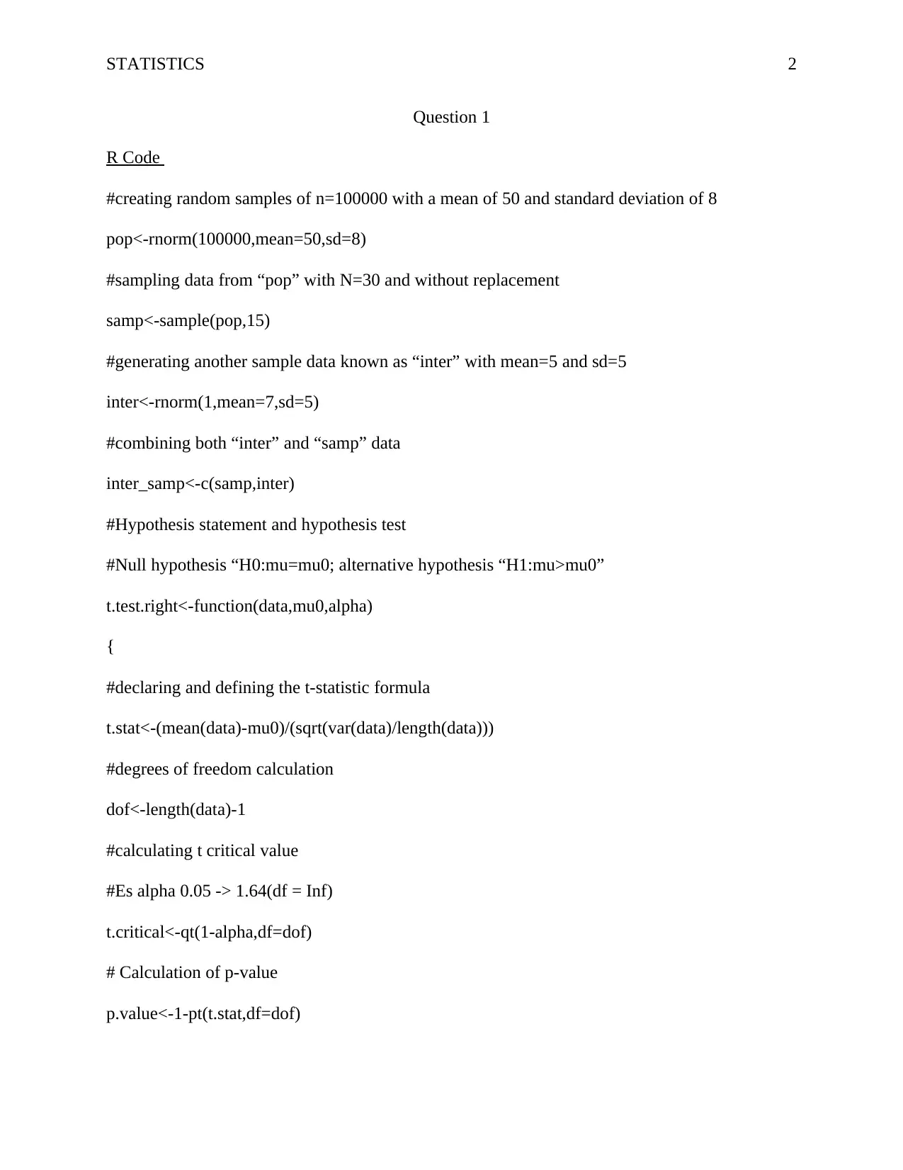
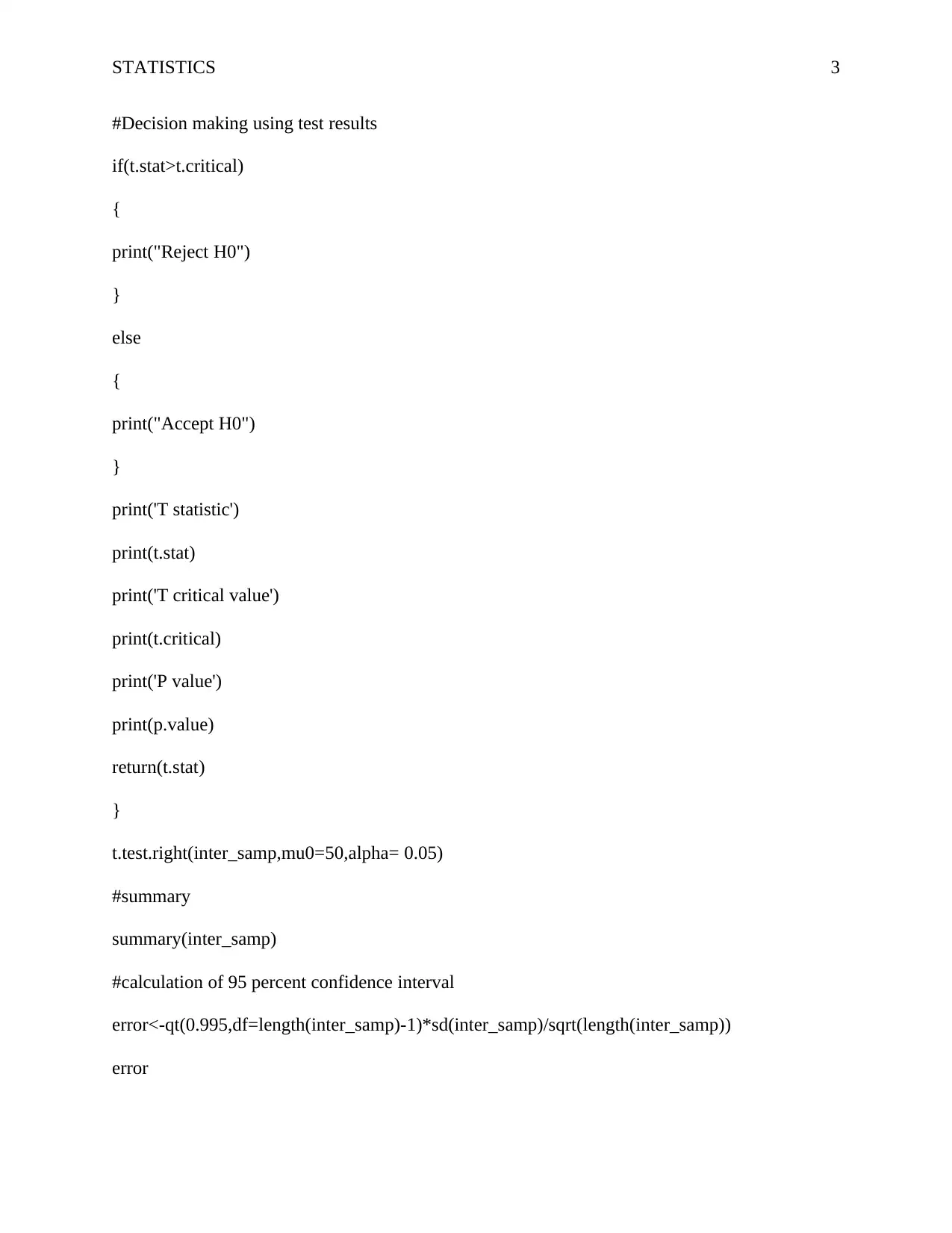
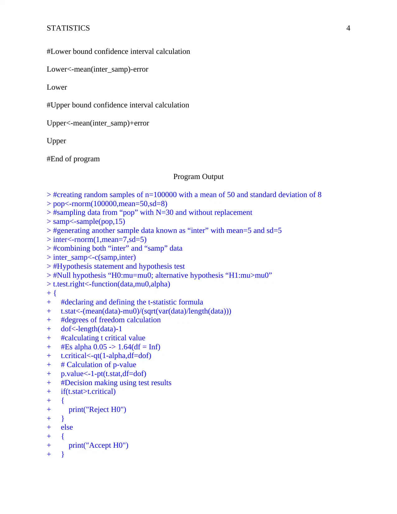
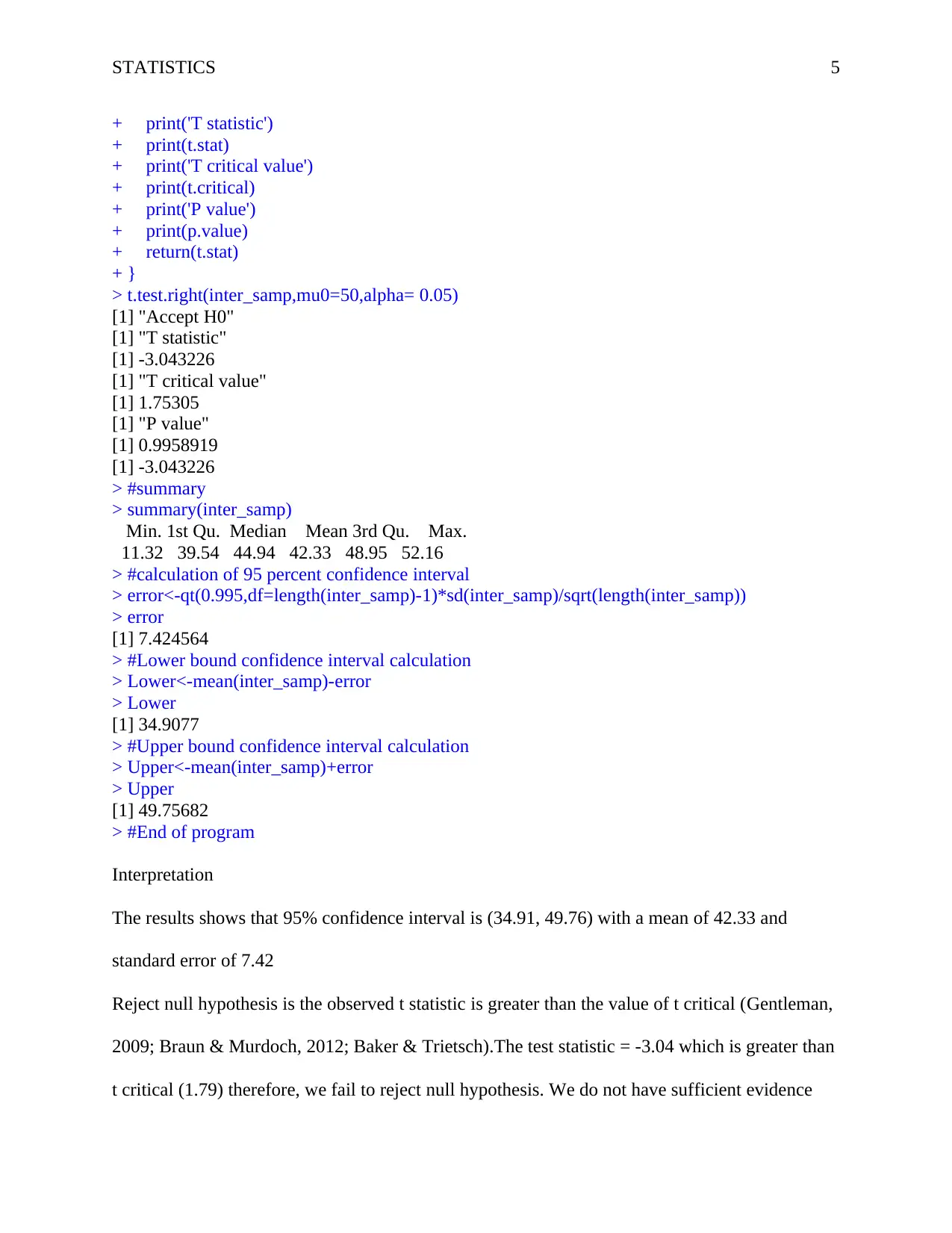
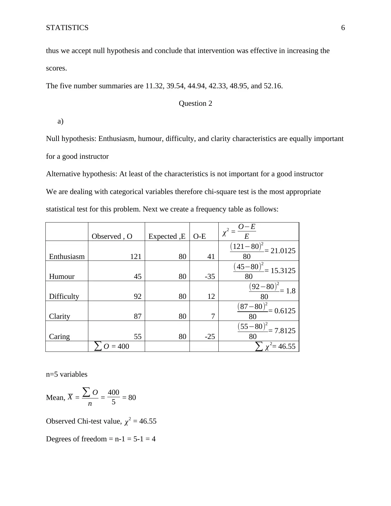
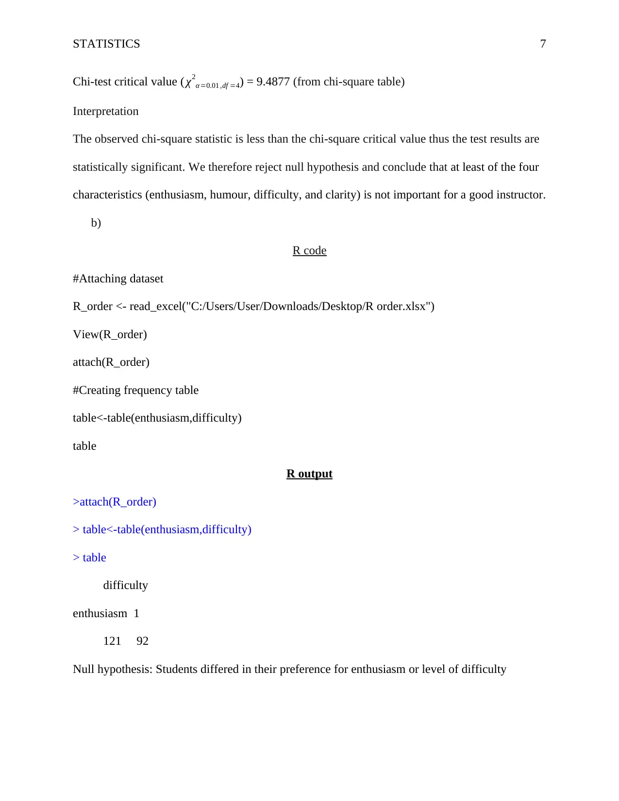
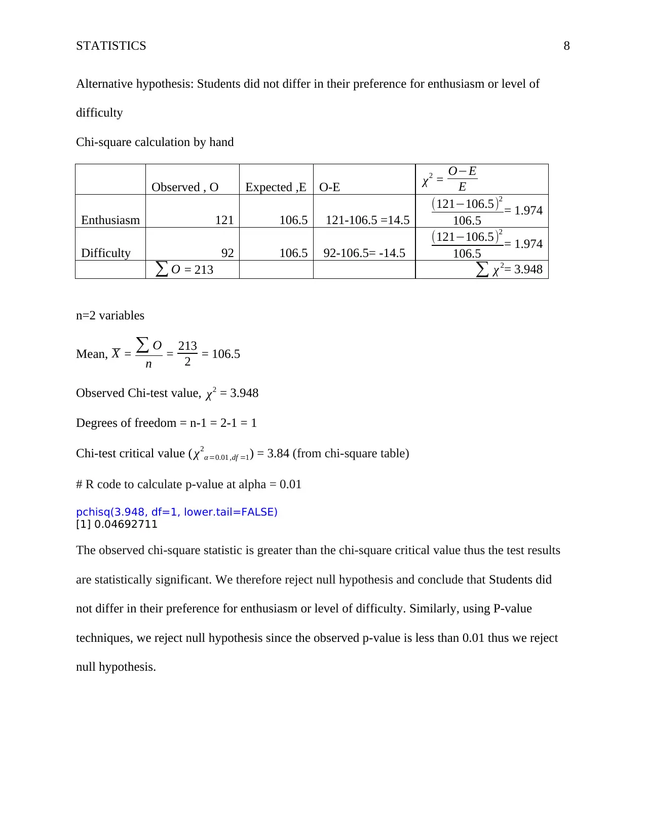
This assignment focuses on statistical methods and hypothesis testing using R. It includes creating a normally distributed population, sampling data, performing a t-test to evaluate the effectiveness of an intervention, and conducting a chi-square test to analyze categorical variables. The assignment provides R code, output, and interpretations of the results, including confidence intervals and p-values. It covers both manual calculations and R-based analysis for hypothesis testing, along with interpretations based on critical values and p-values. Desklib is your go-to resource for accessing similar solved assignments and study materials.

Running head: STATISTICS
1
Statistical Methods 1
Student Name
Institution

STATISTICS 2
Question 1
R Code
#creating random samples of n=100000 with a mean of 50 and standard deviation of 8
pop<-rnorm(100000,mean=50,sd=8)
#sampling data from “pop” with N=30 and without replacement
samp<-sample(pop,15)
#generating another sample data known as “inter” with mean=5 and sd=5
inter<-rnorm(1,mean=7,sd=5)
#combining both “inter” and “samp” data
inter_samp<-c(samp,inter)
#Hypothesis statement and hypothesis test
#Null hypothesis “H0:mu=mu0; alternative hypothesis “H1:mu>mu0”
t.test.right<-function(data,mu0,alpha)
{
#declaring and defining the t-statistic formula
t.stat<-(mean(data)-mu0)/(sqrt(var(data)/length(data)))
#degrees of freedom calculation
dof<-length(data)-1
#calculating t critical value
#Es alpha 0.05 -> 1.64(df = Inf)
t.critical<-qt(1-alpha,df=dof)
# Calculation of p-value
p.value<-1-pt(t.stat,df=dof)

STATISTICS 3
#Decision making using test results
if(t.stat>t.critical)
{
print("Reject H0")
}
else
{
print("Accept H0")
}
print('T statistic')
print(t.stat)
print('T critical value')
print(t.critical)
print('P value')
print(p.value)
return(t.stat)
}
t.test.right(inter_samp,mu0=50,alpha= 0.05)
#summary
summary(inter_samp)
#calculation of 95 percent confidence interval
error<-qt(0.995,df=length(inter_samp)-1)*sd(inter_samp)/sqrt(length(inter_samp))
error

STATISTICS 4
#Lower bound confidence interval calculation
Lower<-mean(inter_samp)-error
Lower
#Upper bound confidence interval calculation
Upper<-mean(inter_samp)+error
Upper
#End of program
Program Output
> #creating random samples of n=100000 with a mean of 50 and standard deviation of 8
> pop<-rnorm(100000,mean=50,sd=8)
> #sampling data from “pop” with N=30 and without replacement
> samp<-sample(pop,15)
> #generating another sample data known as “inter” with mean=5 and sd=5
> inter<-rnorm(1,mean=7,sd=5)
> #combining both “inter” and “samp” data
> inter_samp<-c(samp,inter)
> #Hypothesis statement and hypothesis test
> #Null hypothesis “H0:mu=mu0; alternative hypothesis “H1:mu>mu0”
> t.test.right<-function(data,mu0,alpha)
+ {
+ #declaring and defining the t-statistic formula
+ t.stat<-(mean(data)-mu0)/(sqrt(var(data)/length(data)))
+ #degrees of freedom calculation
+ dof<-length(data)-1
+ #calculating t critical value
+ #Es alpha 0.05 -> 1.64(df = Inf)
+ t.critical<-qt(1-alpha,df=dof)
+ # Calculation of p-value
+ p.value<-1-pt(t.stat,df=dof)
+ #Decision making using test results
+ if(t.stat>t.critical)
+ {
+ print("Reject H0")
+ }
+ else
+ {
+ print("Accept H0")
+ }

STATISTICS 5
+ print('T statistic')
+ print(t.stat)
+ print('T critical value')
+ print(t.critical)
+ print('P value')
+ print(p.value)
+ return(t.stat)
+ }
> t.test.right(inter_samp,mu0=50,alpha= 0.05)
[1] "Accept H0"
[1] "T statistic"
[1] -3.043226
[1] "T critical value"
[1] 1.75305
[1] "P value"
[1] 0.9958919
[1] -3.043226
> #summary
> summary(inter_samp)
Min. 1st Qu. Median Mean 3rd Qu. Max.
11.32 39.54 44.94 42.33 48.95 52.16
> #calculation of 95 percent confidence interval
> error<-qt(0.995,df=length(inter_samp)-1)*sd(inter_samp)/sqrt(length(inter_samp))
> error
[1] 7.424564
> #Lower bound confidence interval calculation
> Lower<-mean(inter_samp)-error
> Lower
[1] 34.9077
> #Upper bound confidence interval calculation
> Upper<-mean(inter_samp)+error
> Upper
[1] 49.75682
> #End of program
Interpretation
The results shows that 95% confidence interval is (34.91, 49.76) with a mean of 42.33 and
standard error of 7.42
Reject null hypothesis is the observed t statistic is greater than the value of t critical (Gentleman,
2009; Braun & Murdoch, 2012; Baker & Trietsch).The test statistic = -3.04 which is greater than
t critical (1.79) therefore, we fail to reject null hypothesis. We do not have sufficient evidence

STATISTICS 6
thus we accept null hypothesis and conclude that intervention was effective in increasing the
scores.
The five number summaries are 11.32, 39.54, 44.94, 42.33, 48.95, and 52.16.
Question 2
a)
Null hypothesis: Enthusiasm, humour, difficulty, and clarity characteristics are equally important
for a good instructor
Alternative hypothesis: At least of the characteristics is not important for a good instructor
We are dealing with categorical variables therefore chi-square test is the most appropriate
statistical test for this problem. Next we create a frequency table as follows:
Observed , O Expected ,E O-E χ2 = O−E
E
Enthusiasm 121 80 41
(121−80)2
80 = 21.0125
Humour 45 80 -35
(45−80)2
80 = 15.3125
Difficulty 92 80 12
(92−80)2
80 = 1.8
Clarity 87 80 7
(87−80)2
80 = 0.6125
Caring 55 80 -25
(55−80)2
80 = 7.8125
∑ O = 400 ∑ χ 2= 46.55
n=5 variables
Mean, X = ∑ O
n = 400
5 = 80
Observed Chi-test value, χ2 = 46.55
Degrees of freedom = n-1 = 5-1 = 4

STATISTICS 7
Chi-test critical value ( χ2
α =0.01 ,df =4) = 9.4877 (from chi-square table)
Interpretation
The observed chi-square statistic is less than the chi-square critical value thus the test results are
statistically significant. We therefore reject null hypothesis and conclude that at least of the four
characteristics (enthusiasm, humour, difficulty, and clarity) is not important for a good instructor.
b)
R code
#Attaching dataset
R_order <- read_excel("C:/Users/User/Downloads/Desktop/R order.xlsx")
View(R_order)
attach(R_order)
#Creating frequency table
table<-table(enthusiasm,difficulty)
table
R output
>attach(R_order)
> table<-table(enthusiasm,difficulty)
> table
difficulty
enthusiasm 1
121 92
Null hypothesis: Students differed in their preference for enthusiasm or level of difficulty

STATISTICS 8
Alternative hypothesis: Students did not differ in their preference for enthusiasm or level of
difficulty
Chi-square calculation by hand
Observed , O Expected ,E O-E χ2 = O−E
E
Enthusiasm 121 106.5 121-106.5 =14.5
(121−106.5)2
106.5 = 1.974
Difficulty 92 106.5 92-106.5= -14.5
(121−106.5)2
106.5 = 1.974
∑ O = 213 ∑ χ 2= 3.948
n=2 variables
Mean, X = ∑ O
n = 213
2 = 106.5
Observed Chi-test value, χ2 = 3.948
Degrees of freedom = n-1 = 2-1 = 1
Chi-test critical value ( χ2
α =0.01 ,df =1) = 3.84 (from chi-square table)
# R code to calculate p-value at alpha = 0.01
pchisq(3.948, df=1, lower.tail=FALSE)
[1] 0.04692711
The observed chi-square statistic is greater than the chi-square critical value thus the test results
are statistically significant. We therefore reject null hypothesis and conclude that Students did
not differ in their preference for enthusiasm or level of difficulty. Similarly, using P-value
techniques, we reject null hypothesis since the observed p-value is less than 0.01 thus we reject
null hypothesis.

STATISTICS 9
References
Baker, K., & Trietsch, D.(2009) Principles of sequencing and scheduling.
Braun, J., & Murdoch, D.(2012). A first course in statistical programming with R.
Gentleman, R. (2009). R programming for bioinformatics. Boca Raton: CRC Press.