BUS708 Statistical Modelling Assignment: NSW Transport System Analysis

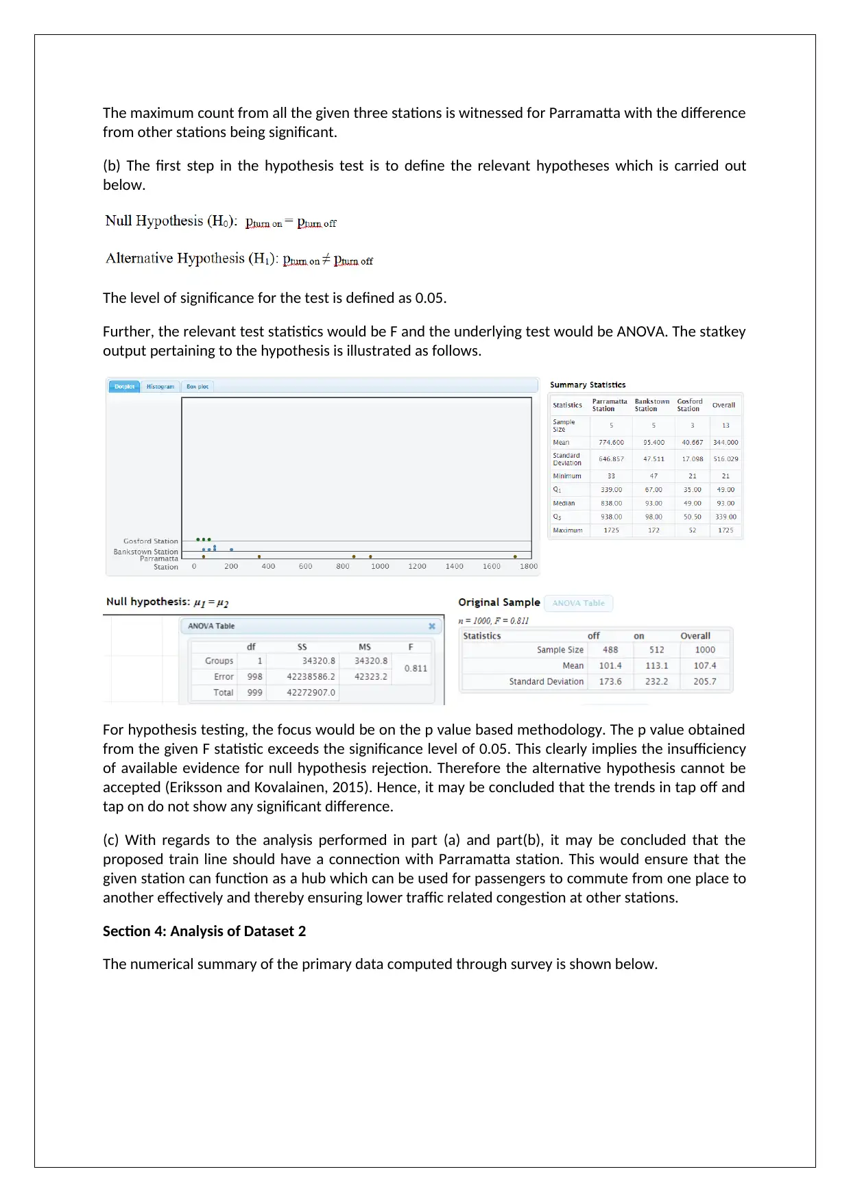
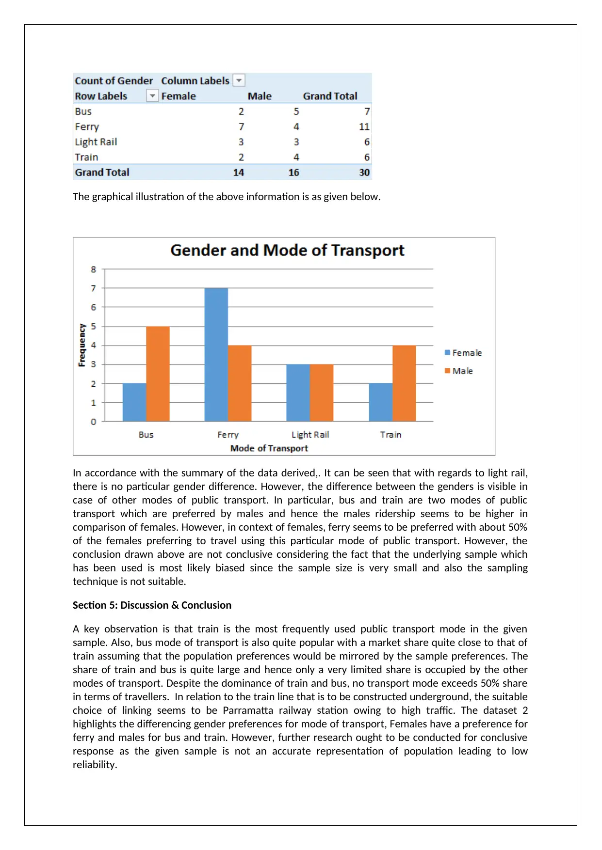
This report presents a comprehensive analysis of the NSW transport system using statistical modeling techniques, based on the BUS708 assignment. The report begins with an introduction, providing context and defining the datasets used: Dataset 1 (secondary data) and Dataset 2 (primary data). It then proceeds to analyze single variables within Dataset 1, focusing on the usage of different public transport modes, and performs hypothesis testing to determine the share of train usage. The analysis extends to two variables in Dataset 1, examining the relationship between train usage and different stations, also including hypothesis testing. Finally, the report analyzes Dataset 2, focusing on gender preferences for different transport modes, and concludes with a discussion of findings, limitations, and recommendations for future research, including the suggestion of connecting Parramatta station to the proposed train line.

STATISTICAL MODELLING
STUDENT ID:
[Pick the date]

Section 1: Introduction
a) In cities, a crucial challenge for planners is to ensure that the transport infrastructure must be
robust to cater to the ever increasing population while ensuring efficiency and also affordability
that is associated with public transport system. For enabling the same, the relevant authority
tends to make changes in route of timetable and stoppages so that the available infrastructure
can be utilised more efficiently and serve greater number of people. In this regards, some of the
people may be negatively impacted but the larger good is considered more important. As a
result, the decision to change timetable and stoppages must be taken after due research from
specialised agencies who understand the preferences and the issues faced by the travellers
(Meyers, 2017).
b) In order to determine whether the given dataset is primary or not, it needs to be seen if the
underlying data has been collected by the entity conducting the research. It is apparent that the
given data in dataset 1 has neither been collected by myself nor has been collected by the
university. This data was computed by an external agency and hence the given dataset 1 would
be termed as secondary data (Eriksson and Kovalainen, 2015). The given dataset has an
underlying sample size of 1000 observations and the given information is represented in the form
of six variables. For the variables such as location, tap, mode the underlying data type is
categorical and since automatic arrangements of the respective values is not possible; hence the
applicable measurement scale is nominal. On the other hand, date is also a categorical variable
but the underlying measurement type of ordinal since arrangement in an orderly manner without
any additional information is possible. Count and time are both quantitative variables, however
the relevant measurement scale for the former would be ratio while for the latter would be
interval (Flick, 2015). The cases in the dataset would correspond to a tap on or tap off at a given
location at a given time through a defined mode on a particular date. The frequency of each of
these cases is represented using the count variable.
c) The dataset 2 is a primary data since it has been obtained from any source but rather has been
collected through the use of survey (Hair et. al., 2015).. The focus of the survey was only on
recording two variables namely the preferred mode of public transport coupled with the underlying
gender of the respondent. Even though dataset 2 is primary data unlike dataset 1, but this would
not automatically imply that the former is more accurate than the latter. For the reliability of data
obtained from primary source, the sample needs to representative of the underlying population.
This is clearly not the case because of the following two reasons (Eriksson and Kovalainen, 2015).
 The sample size is only 30 which is very small compared the population and the key
attributes driving the preferences.
 Random sampling is not deployed and instead the sample selection has been done based on
convenience.
In the given case, the two variables i.e. transport mode and gender are variables of categorical form
with a nominal measurement scale (Hillier, 2016).
Section 2: Single variable Analysis – Dataset 1
a) The usage of public transport numerical summary for the given sample data is as shown below.

The graphical illustration of the above information is as given below.
As per the given summary table and graph regarding the transport mode, it is apparent that the
mode which is most frequently used is train as is clear from the sample data where it has the
maximum frequency. However, bus mode is also quite close and trails by only a minimal insignificant
difference. But the contribution of other means of transport besides bus and train is only 5% thereby
indicating a high degree of reliance on bus and train in the public transport system. As a result, going
forward it is desired that relevant measures must be undertaken to strengthen the bus and train
infrastructure so that it can handle higher number of passengers. Alternatively, the other means of
public transport should be explored so as to ease the pressure and underlying traffic on bus and
train.
b) The first step in the hypothesis test is to define the relevant hypotheses which is carried out
below.
The level of significance for the test is defined as 0.05.

Further, the relevant test statistics would be Z and the underlying test would be a one tail test. The
excel output pertaining to the hypothesis is illustrated as follows.
For hypothesis testing, the focus would be on the p value based methodology. The p value obtained
is 0.93 and hence exceeds the significance level of 0.05. This clearly implies the insufficiency of
available evidence for null hypothesis rejection (Flick, 2015). Therefore the alternative hypothesis
cannot be accepted. This hints that train does not have a share of over 50% in the public transport in
NSW.
Section 3: Analysis of Two Variables – Dataset 1
a) The public transport train related numerical summary in relation to three chosen stations for the
given sample data is as shown below.
The graphical illustration of the above information is as given below.

The maximum count from all the given three stations is witnessed for Parramatta with the difference
from other stations being significant.
(b) The first step in the hypothesis test is to define the relevant hypotheses which is carried out
below.
The level of significance for the test is defined as 0.05.
Further, the relevant test statistics would be F and the underlying test would be ANOVA. The statkey
output pertaining to the hypothesis is illustrated as follows.
For hypothesis testing, the focus would be on the p value based methodology. The p value obtained
from the given F statistic exceeds the significance level of 0.05. This clearly implies the insufficiency
of available evidence for null hypothesis rejection. Therefore the alternative hypothesis cannot be
accepted (Eriksson and Kovalainen, 2015). Hence, it may be concluded that the trends in tap off and
tap on do not show any significant difference.
(c) With regards to the analysis performed in part (a) and part(b), it may be concluded that the
proposed train line should have a connection with Parramatta station. This would ensure that the
given station can function as a hub which can be used for passengers to commute from one place to
another effectively and thereby ensuring lower traffic related congestion at other stations.
Section 4: Analysis of Dataset 2
The numerical summary of the primary data computed through survey is shown below.

The graphical illustration of the above information is as given below.
In accordance with the summary of the data derived,. It can be seen that with regards to light rail,
there is no particular gender difference. However, the difference between the genders is visible in
case of other modes of public transport. In particular, bus and train are two modes of public
transport which are preferred by males and hence the males ridership seems to be higher in
comparison of females. However, in context of females, ferry seems to be preferred with about 50%
of the females preferring to travel using this particular mode of public transport. However, the
conclusion drawn above are not conclusive considering the fact that the underlying sample which
has been used is most likely biased since the sample size is very small and also the sampling
technique is not suitable.
Section 5: Discussion & Conclusion
A key observation is that train is the most frequently used public transport mode in the given
sample. Also, bus mode of transport is also quite popular with a market share quite close to that of
train assuming that the population preferences would be mirrored by the sample preferences. The
share of train and bus is quite large and hence only a very limited share is occupied by the other
modes of transport. Despite the dominance of train and bus, no transport mode exceeds 50% share
in terms of travellers. In relation to the train line that is to be constructed underground, the suitable
choice of linking seems to be Parramatta railway station owing to high traffic. The dataset 2
highlights the differencing gender preferences for mode of transport, Females have a preference for
ferry and males for bus and train. However, further research ought to be conducted for conclusive
response as the given sample is not an accurate representation of population leading to low
reliability.

It is quite possible that the trends and preferences of travellers may be influenced by some
extraneous factor during the given period. Hence, in order to draw more reliable conclusions, data
should be taken on more dates of different months so as to ensure that the preferences are clearer.
This is required considering the high degree of capital investment that is required in enabling
infrastructure for bus and train.

References
Eriksson, P. and Kovalainen, A. (2015) Quantitative methods in business research 3rd ed. London:
Sage Publications.
Flick, U. (2015) Introducing research methodology: A beginner's guide to doing a research project.
4th ed. New York: Sage Publications.
Hair, J. F., Wolfinbarger, M., Money, A. H., Samouel, P., and Page, M. J. (2015) Essentials of business
research methods. 2nd ed. New York: Routledge.
Hillier, F. (2016) Introduction to Operations Research 6th ed. New York: McGraw Hill Publications.
Mayers, L. (2017) Greater Sydney and NSW public transport undergo state's 'largest' timetable
overhaul ever, [online] Available at http://www.abc.net.au/news/2017-11-26/new-sydney-and-nsw-
public-transport-timetable-launched/9194538 (Assessed September 19, 2018)