Statistical Modelling: Model Construction, ANN Training & Problems

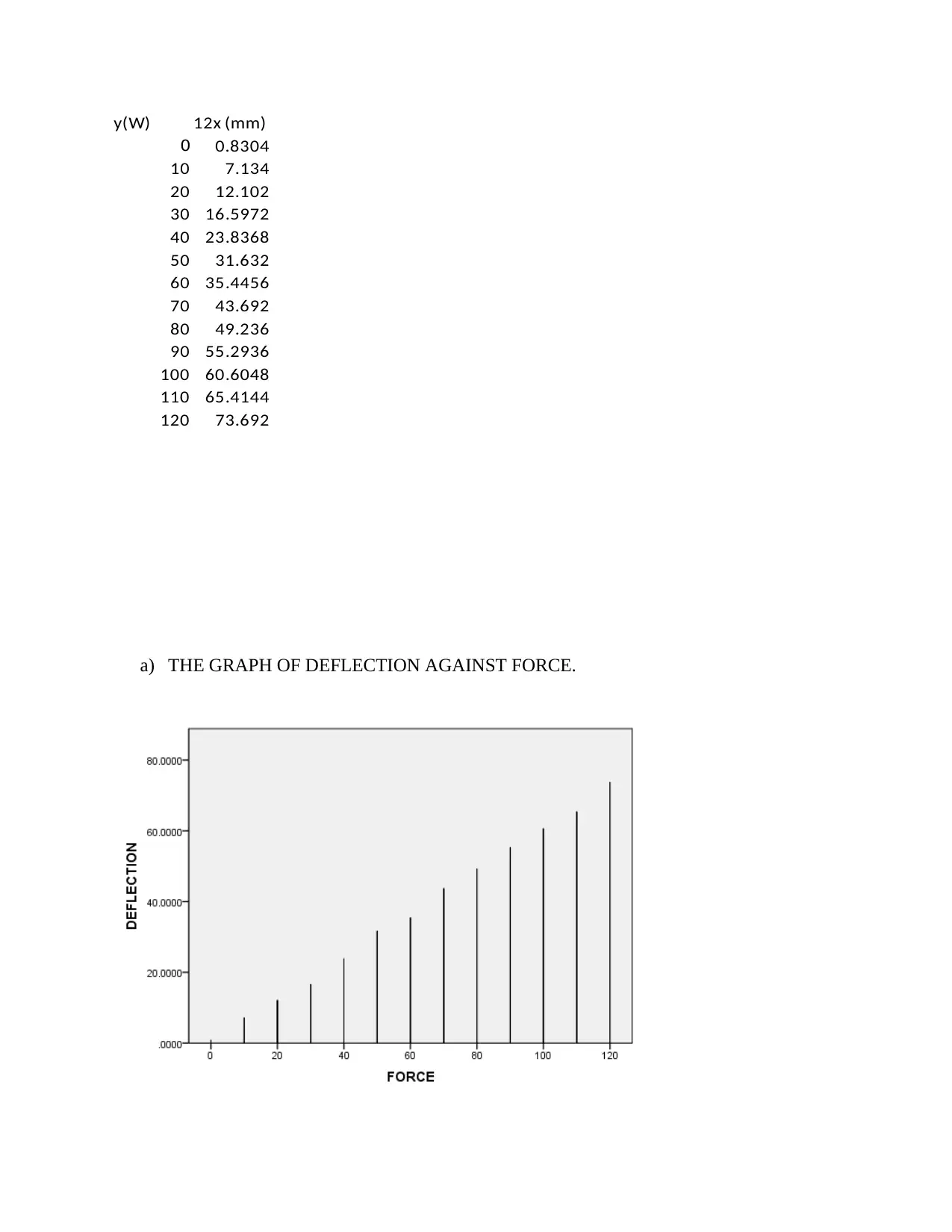
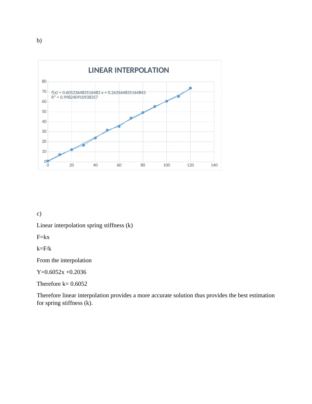
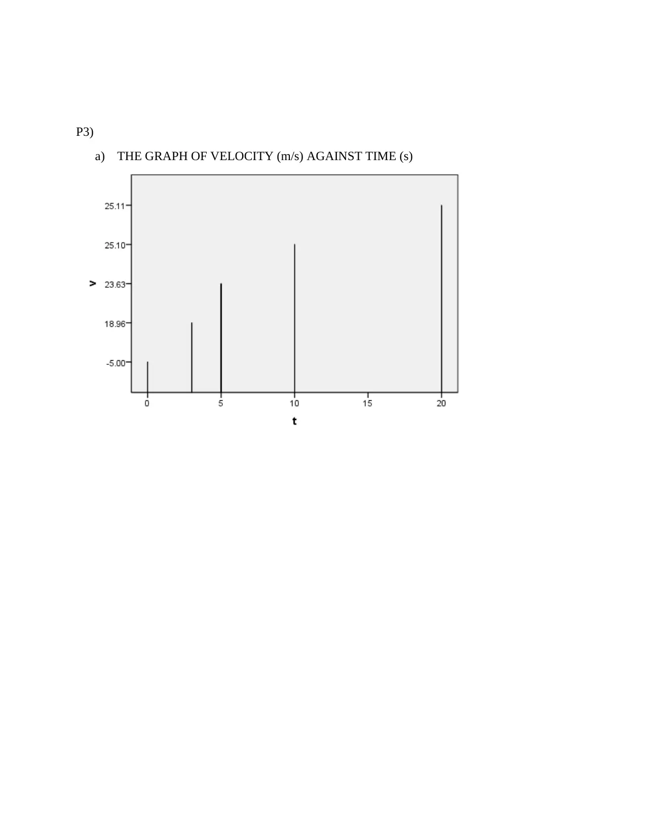
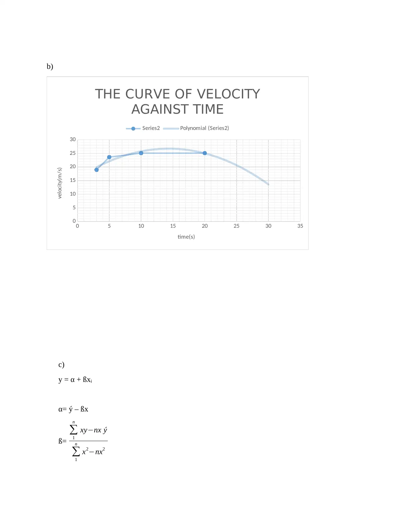
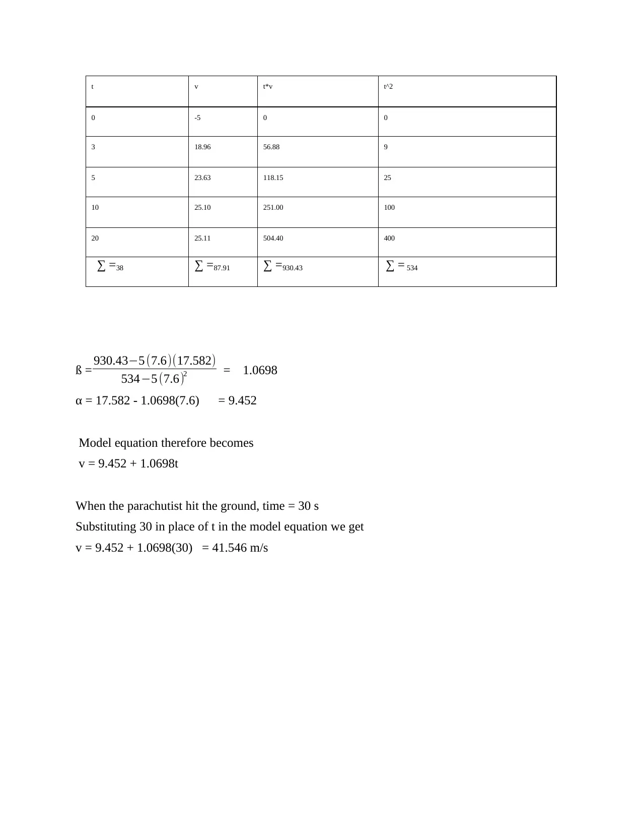
This document presents a comprehensive solution to a statistical modelling assignment. It covers the process of constructing a mathematical model, including problem identification, assumption making, model solving, verification, implementation, and maintenance. The solution also discusses data-driven modelling, model fitting, and the training of Artificial Neural Networks (ANNs). Furthermore, it includes detailed solutions to specific problems involving interest calculations, linear interpolation for spring stiffness estimation, and regression analysis for modelling velocity against time. The document provides graphs, equations, and explanations to support the solutions, offering a thorough understanding of the concepts and techniques involved in statistical modelling.

STATISTICAL MODELLING
By (Name)
Course Name
Name of the Professor
Student’s Name
Date

Q1)
The process of constructing a Mathematical model.
i) Problem identification – This is the first step in model building. Here, the
problem in question is identified or identification of the main aim of
developing a model. It identifies the main necessities for constructing the
model.
ii) Make assumptions –This involves making claims about the model. This step
entails the identification and classification of the variable of interest to be
used. At this stage, dependent and independent variables are distinguished.
iii) Solving or interpreting the model –After all the variables of interest have been
identified and classified, the next step is to solve the model. This is done by
determining the relationship between the variables and sub-models developed.
This will provide an easy way to interpret the model as the relationships
between variables are clearly distinguished in this stage.
iv) Mode verification – This is the assessing or evaluating the appropriateness of
the model whether it is really giving the solution to the said problem and also
whether it makes sense.This is typically done by checking whether a model
fits exploratory estimations or other observational information. In models with
parameters, a typical way to deal with the test this fit is to part the information
into two disjoint subsets: preparing information and check information. The
preparation information is utilized to appraise the model parameters. A precise
model will intently coordinate the confirmation information. It can likewise be
tried with certifiable information. On the off chance that the model isn't
alluring, at that point different models are created until the best one is
acquired which is then considered.Implementation of the model – After the
model has been tested and verified to be fit, the model is then implemented to
be used. In this stage, the model is free from errors and is ready to be
implemented.
v) Maintaining the model – This is the last stage in model construction. It
majorly involves regular checking and validation of the model to ensure it is
fit at all times.
a) Verification is the process of confirming whether the model is correctly
implemented based on specifications and assumptions deemed applicable.
This is done by making logical flow diagrams, assessing the reasonability

of the model output by the experts and the use of debugger software. The
model can also be subjected to dry-running so as to ensure its correctness.
b) Validation is the process of checking the accuracy of the model compared
to the real world data.
Q2) data-driven modeling
A data-driven demonstrating is the displaying that envelops experimental methodologies (linear
regression, machine learning, ARIMA models) in view of breaking down the information about
the framework by discovering an association with the framework state factors (input, internal and
output variables) without unequivocal learning of the physical conduct.
Model fitting is the way toward building a bend that has the most elevated exactness of fit to the
arrangement of information point. Information fitting is characterized as the way toward fitting
models to information and dissecting the level of exactness of the fit. In information fitting,
information methods including scientific conditions and nonparametric conditions are utilized.
Model fitting then again makes utilization of parametric conditions.
Q3) Training of Artificial Neural Networks (ANNs)
Preparing of Artificial Neural Network (ANNs) alludes to the way toward preparing a system
that has been organized for a specific application in order to speak to the connections and
procedures that are natural inside the information. When the systems are prepared to fulfillment,
it very well may be put to task when the new info information are gone through the prepared
system in its non-preparing mode to deliver the ideal model yields.
Preparing ANNs is firmly identified with a relapse in that they play out an information yield
mapping utilizing a lot of interconnected basic handling hubs or neurons. Every neuron takes in
data sources either remotely or from different neurons and goes it through an enactment or
exchange capacity, for example, a strategic or sigmoid bend. Information enters the system
through the information units organized in what is called an information layer. This information
is then sustained forward through progressive layers incorporating the concealed layer in the
center to rise up out of the yielding layer on the right. The data sources can be any blend of
factors that are believed to be critical for anticipating the yield; accordingly, some learning of the
hydrological framework is essential.
P1)
a)
SID =15
Total months (T) = (15 × 4) + 36 = 96
Total amount payable = P + I
Where P = Principle, I = interest.

I = A – P
A= P (1 + r
100 )^n
Where r is the interest rate, n = the number of months.
Hr1 =0.16% , r2 =0.35%
T = t1 + t2 = 96
Gt1= 24, t2= T –t1 = 96 -24 =72
P = £ 1300,000
A1= £ 1300,000 (1 + 0.16
100 )^24 = 1350849.397
A2 = £ 1300,000 (1 + 0.35
100 ¿^72 = 1671839.121
I1 = 1350849.397 - 1300,000 = 50849.397
I2 = 1671839.121 - 1300,000 = 371839.1214
I = I1 +I2 = 50849.397 +371839.1214 = 422688.5184
TA = P + I = £ 1300,000 + 422688.5184 = 1722688.518
Hence total amount payable at the end of 96 months is 1722688.518
Payments per month = A
T = 1722688.518
96 = 17944.67206
b)
t = 30,
= (1722688.518 × 30) = 538338.618
Outstanding balance = 1722688.518 - 538338.618 = 1184349.9
P2)
Last three student id digits = 515.
Scaling factor = 5 + 1 + 5 + 1 =12

y(W) 12x (mm)
0 0.8304
10 7.134
20 12.102
30 16.5972
40 23.8368
50 31.632
60 35.4456
70 43.692
80 49.236
90 55.2936
100 60.6048
110 65.4144
120 73.692
a) THE GRAPH OF DEFLECTION AGAINST FORCE.

b)
0 20 40 60 80 100 120 140
0
10
20
30
40
50
60
70
80
f(x) = 0.605236483516483 x + 0.263564835164843
R² = 0.998240910938357
LINEAR INTERPOLATION
c)
Linear interpolation spring stiffness (k)
F=kx
k=F/k
From the interpolation
Y=0.6052x +0.2036
Therefore k= 0.6052
Therefore linear interpolation provides a more accurate solution thus provides the best estimation
for spring stiffness (k).

P3)
a) THE GRAPH OF VELOCITY (m/s) AGAINST TIME (s)

b)
0 5 10 15 20 25 30 35
0
5
10
15
20
25
30
THE CURVE OF VELOCITY
AGAINST TIME
Series2 Polynomial (Series2)
time(s)
velocity(m/s)
c)
y = α + ßxi
α= ý – ßx
ß=
∑
1
n
xy−nx ý
∑
1
n
x2−nx2

t v t*v t^2
0 -5 0 0
3 18.96 56.88 9
5 23.63 118.15 25
10 25.10 251.00 100
20 25.11 504.40 400
∑ =38 ∑ =87.91 ∑ =930.43 ∑ = 534
ß = 930.43−5 (7.6)(17.582)
534−5 (7.6)2 = 1.0698
α = 17.582 - 1.0698(7.6) = 9.452
Model equation therefore becomes
v = 9.452 + 1.0698t
When the parachutist hit the ground, time = 30 s
Substituting 30 in place of t in the model equation we get
v = 9.452 + 1.0698(30) = 41.546 m/s

Bibliography
Abebe AJ, Price RK (2004) Information theory and neural networks for managing
uncertainty in flood routing. ASCE Journal of Computing in Civil Engineering 18(4): 373–380.
Bhattacharya B, Solomatine DP (2005) Neural networks and M5 model trees in modeling
water level – discharge relationship. Neurocomputing 63: 381–396.
Takagi T, Sugeno M (1985) Fuzzy identification of systems and its applications to
modeling and control. IEEE Transactions on Systems, Man, and Cybernetic SMC-15: 116–132.
Solomatine DP, Dulal KN (2003) Model tree as an alternative to the neural network in
rainfall-runoff modeling. Hydrological Sciences J. 48(3): 399–411.
Konishi, S.; Kitagawa, G. (2008), Information Criteria and Statistical Modeling,
Springer.
Burnham, K. P.; Anderson, D. R. (2002), Model Selection and Multimodel
Inference (2nd ed.), Springer-Verlag.