ECON 380: Comprehensive Solutions to Statistical Problems

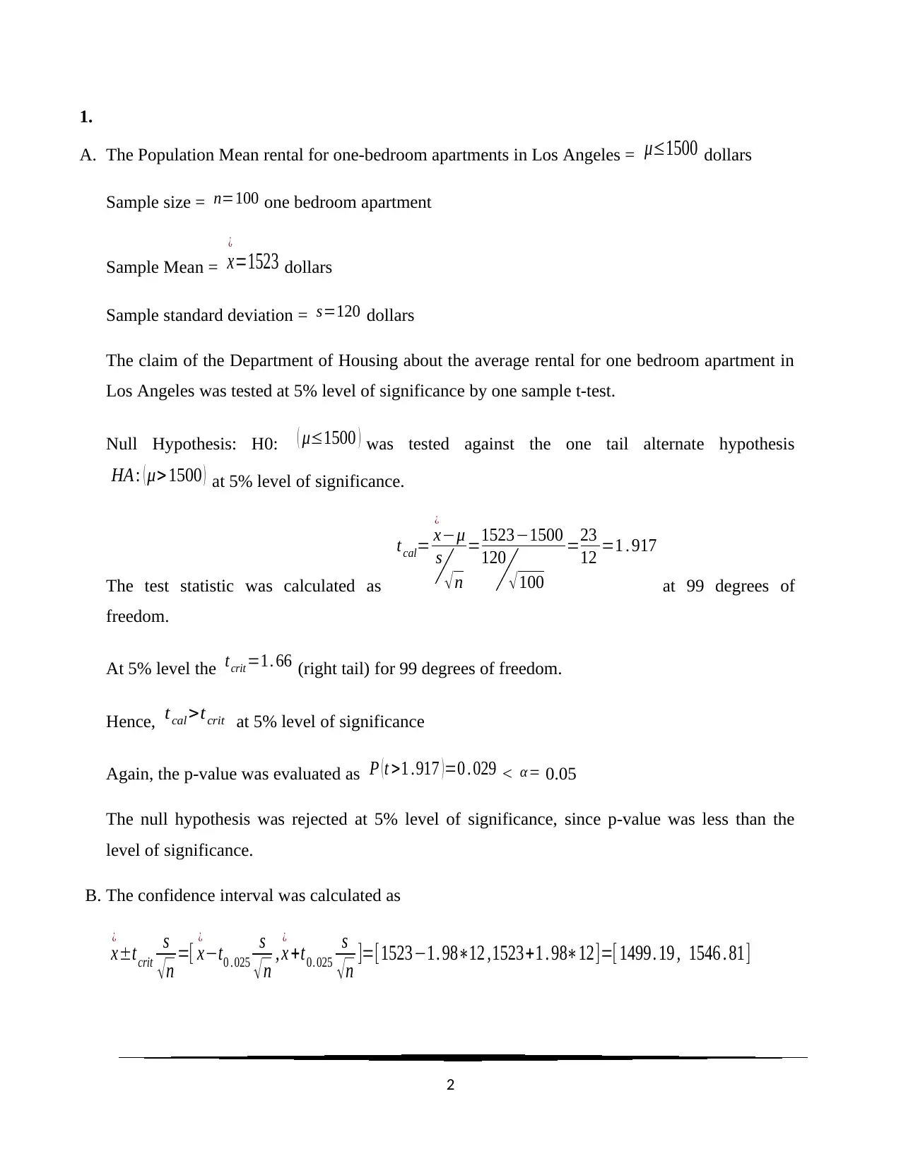
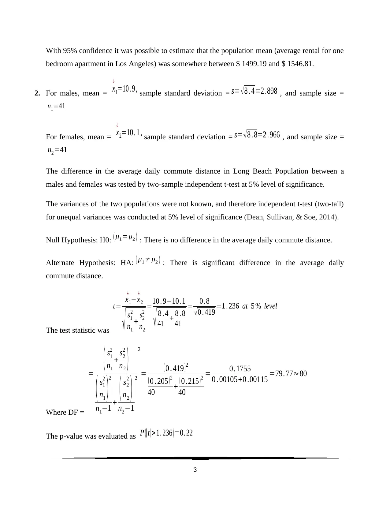
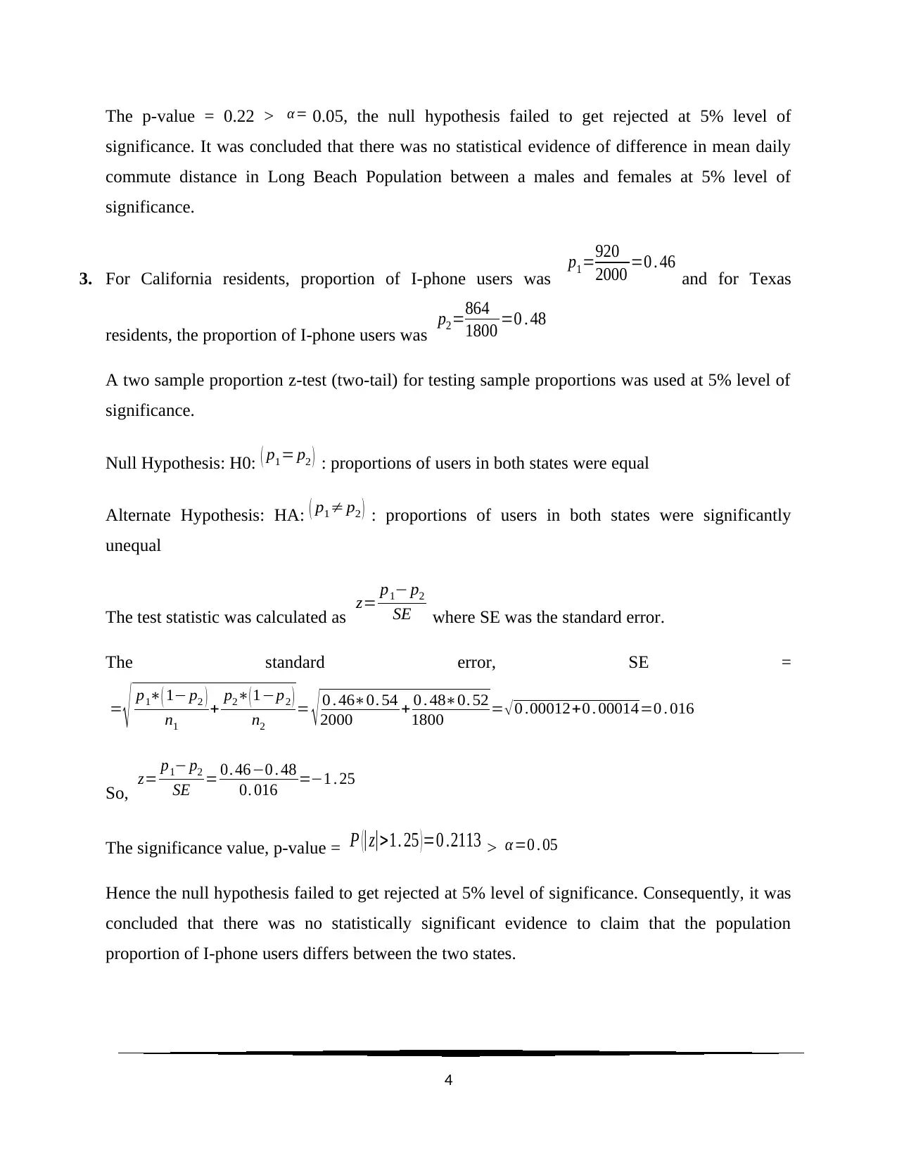
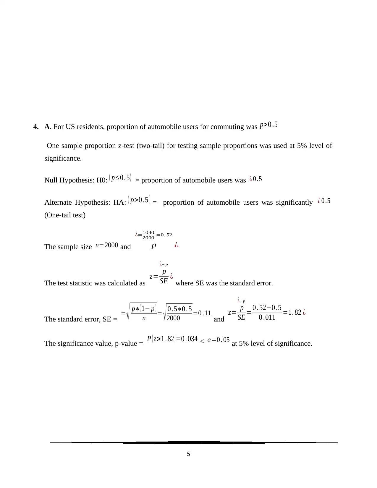
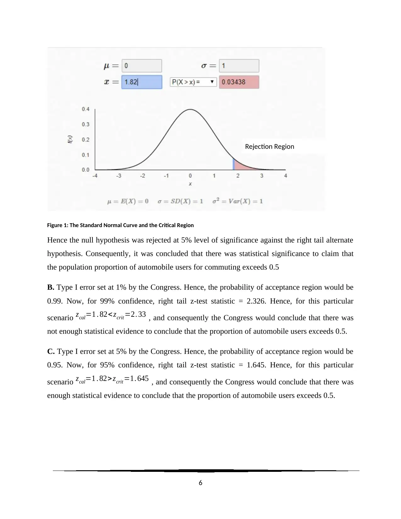
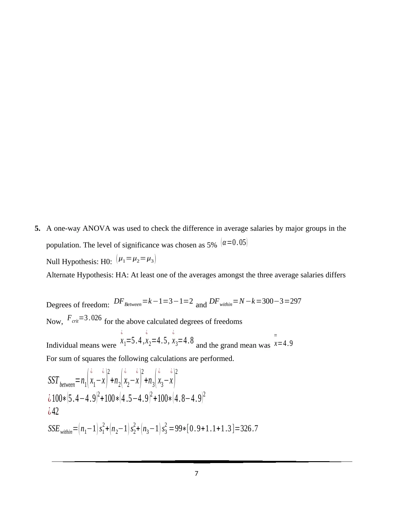
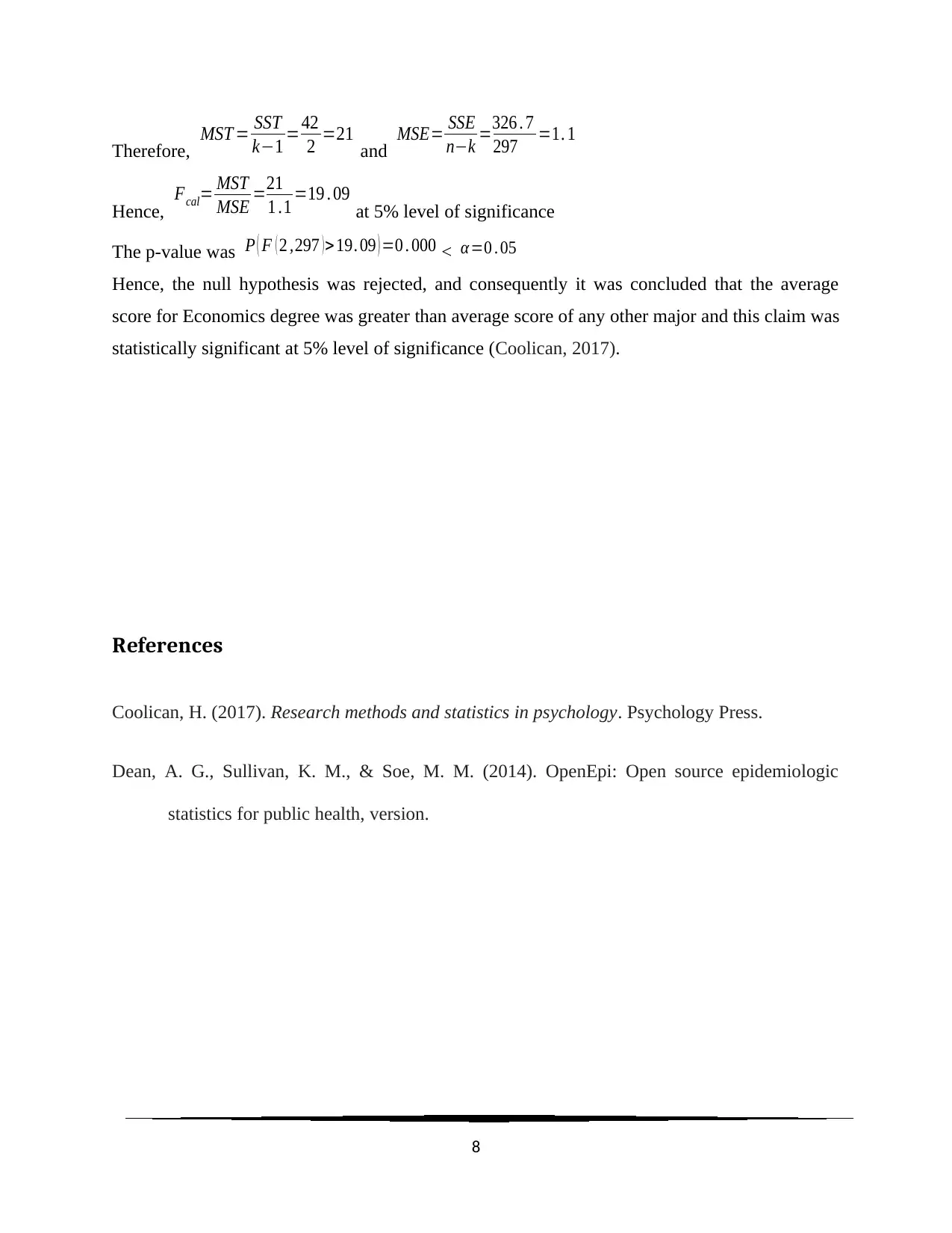
This document provides detailed solutions to several statistical problems. The problems cover a range of topics including one-sample t-tests to test claims about population means, two-sample independent t-tests to compare means between two groups, two-sample proportion z-tests to compare proportions, and one-sample proportion z-tests to test claims about population proportions. Additionally, a one-way ANOVA is used to check for differences in average salaries across different major groups. Each solution includes the null and alternative hypotheses, the calculation of test statistics, determination of p-values, and conclusions based on a 5% level of significance. The document also addresses Type I errors and their implications in decision-making. Desklib offers a platform for students to access similar solved assignments and past papers for academic support.

Statistical Problems
1

1.
A. The Population Mean rental for one-bedroom apartments in Los Angeles = μ≤1500 dollars
Sample size = n=100 one bedroom apartment
Sample Mean = x
¿
=1523 dollars
Sample standard deviation = s=120 dollars
The claim of the Department of Housing about the average rental for one bedroom apartment in
Los Angeles was tested at 5% level of significance by one sample t-test.
Null Hypothesis: H0: ( μ≤1500 ) was tested against the one tail alternate hypothesis
HA : ( μ> 1500 ) at 5% level of significance.
The test statistic was calculated as
tcal= x
¿
−μ
s
√ n
=1523−1500
120
√ 100
=23
12 =1 . 917
at 99 degrees of
freedom.
At 5% level the tcrit =1. 66 (right tail) for 99 degrees of freedom.
Hence, tcal >tcrit at 5% level of significance
Again, the p-value was evaluated as P ( t >1 .917 ) =0 . 029 < α = 0.05
The null hypothesis was rejected at 5% level of significance, since p-value was less than the
level of significance.
B. The confidence interval was calculated as
x
¿
±tcrit
s
√ n =[ x
¿
−t0 . 025
s
√ n , x
¿
+t0. 025
s
√ n ]=[1523−1. 98∗12 ,1523+1 . 98∗12]=[ 1499. 19 , 1546 . 81]
2

With 95% confidence it was possible to estimate that the population mean (average rental for one
bedroom apartment in Los Angeles) was somewhere between $ 1499.19 and $ 1546.81.
2. For males, mean = x
¿
1=10 . 9 , sample standard deviation = s= √ 8 . 4=2 .898 , and sample size =
n1=41
For females, mean = x
¿
2=10 . 1 , sample standard deviation = s= √ 8 . 8=2 . 966 , and sample size =
n2=41
The difference in the average daily commute distance in Long Beach Population between a
males and females was tested by two-sample independent t-test at 5% level of significance.
The variances of the two populations were not known, and therefore independent t-test (two-tail)
for unequal variances was conducted at 5% level of significance (Dean, Sullivan, & Soe, 2014).
Null Hypothesis: H0: ( μ1=μ2 ) : There is no difference in the average daily commute distance.
Alternate Hypothesis: HA: ( μ1≠μ2 ) : There is significant difference in the average daily
commute distance.
The test statistic was
t = x1
¿
−x
¿
2
√ s1
2
n1
+ s2
2
n2
=10 . 9−10 .1
√ 8 . 4
41 + 8 . 8
41
= 0 .8
√ 0 . 419 =1 . 236 at 5 % level
Where DF =
=
( s1
2
n1
+ s2
2
n2 )
( s1
2
n1 )
2
n1−1 +
( s2
2
n2 )
n2−1
2
2
= ( 0 . 419 ) 2
( 0 . 205 ) 2
40 + ( 0 .215 ) 2
40
= 0. 1755
0 . 00105+0 .00115 =79. 77≈80
The p-value was evaluated as P (|t|> 1. 236 ) =0. 22
3

The p-value = 0.22 > α = 0.05, the null hypothesis failed to get rejected at 5% level of
significance. It was concluded that there was no statistical evidence of difference in mean daily
commute distance in Long Beach Population between a males and females at 5% level of
significance.
3. For California residents, proportion of I-phone users was p1=920
2000 =0 . 46 and for Texas
residents, the proportion of I-phone users was p2=864
1800 =0 . 48
A two sample proportion z-test (two-tail) for testing sample proportions was used at 5% level of
significance.
Null Hypothesis: H0: ( p1= p2 ) : proportions of users in both states were equal
Alternate Hypothesis: HA: ( p1≠ p2 ) : proportions of users in both states were significantly
unequal
The test statistic was calculated as z= p1− p2
SE where SE was the standard error.
The standard error, SE =
= √ p1∗( 1− p2 )
n1
+ p2∗( 1−p2 )
n2
= √ 0 . 46∗0. 54
2000 + 0 . 48∗0. 52
1800 = √ 0 .00012+0 . 00014=0 . 016
So, z= p1− p2
SE = 0. 46−0 . 48
0. 016 =−1 . 25
The significance value, p-value = P (|z|>1. 25 ) =0 .2113 > α=0 . 05
Hence the null hypothesis failed to get rejected at 5% level of significance. Consequently, it was
concluded that there was no statistically significant evidence to claim that the population
proportion of I-phone users differs between the two states.
4

4. A. For US residents, proportion of automobile users for commuting was p>0 .5
One sample proportion z-test (two-tail) for testing sample proportions was used at 5% level of
significance.
Null Hypothesis: H0: ( p≤0 . 5 ) = proportion of automobile users was ¿ 0 .5
Alternate Hypothesis: HA: ( p>0 .5 ) = proportion of automobile users was significantly ¿ 0 .5
(One-tail test)
The sample size n=2000 and p
^¿=1040
2000 =0. 52
¿
The test statistic was calculated as z= p
^¿− p
SE ¿ where SE was the standard error.
The standard error, SE = = √ p∗( 1− p )
n = √ 0 .5∗0 . 5
2000 =0 .11 and z= p
^¿− p
SE = 0 . 52−0 .5
0 .011 =1. 82 ¿
The significance value, p-value = P ( z >1 . 82 ) =0 . 034 < α=0 . 05 at 5% level of significance.
5

Figure 1: The Standard Normal Curve and the Critical Region
Hence the null hypothesis was rejected at 5% level of significance against the right tail alternate
hypothesis. Consequently, it was concluded that there was statistical significance to claim that
the population proportion of automobile users for commuting exceeds 0.5
B. Type I error set at 1% by the Congress. Hence, the probability of acceptance region would be
0.99. Now, for 99% confidence, right tail z-test statistic = 2.326. Hence, for this particular
scenario zcal=1 . 82< zcrit =2. 33 , and consequently the Congress would conclude that there was
not enough statistical evidence to conclude that the proportion of automobile users exceeds 0.5.
C. Type I error set at 5% by the Congress. Hence, the probability of acceptance region would be
0.95. Now, for 95% confidence, right tail z-test statistic = 1.645. Hence, for this particular
scenario zcal=1 . 82> zcrit =1. 645 , and consequently the Congress would conclude that there was
enough statistical evidence to conclude that the proportion of automobile users exceeds 0.5.
6
Rejection Region

5. A one-way ANOVA was used to check the difference in average salaries by major groups in the
population. The level of significance was chosen as 5% ( α=0 . 05 )
Null Hypothesis: H0: ( μ1=μ2=μ3 )
Alternate Hypothesis: HA: At least one of the averages amongst the three average salaries differs
Degrees of freedom: DFBetween=k −1=3−1=2 and DFwithin=N −k =300−3=297
Now, Fcrit=3 . 026 for the above calculated degrees of freedoms
Individual means were x
¿
1=5 . 4 , x
¿
2=4 . 5 , x
¿
3=4 . 8 and the grand mean was x
=
=4 . 9
For sum of squares the following calculations are performed.
SST between=n1 ( x
¿
1−x
¿
)
2
+n2 ( x
¿
2−x
¿
)
2
+n3 ( x
¿
3−x
¿
)
2
¿ 100∗ ( 5 . 4−4 . 9 ) 2+100∗( 4 .5−4 . 9 )2 +100∗ ( 4 . 8−4 . 9 ) 2
¿ 42
SSEwithin= ( n1−1 ) s1
2+ ( n2−1 ) s2
2+ ( n3−1 ) s3
2 =99∗[0 . 9+1 .1+1 .3 ]=326 .7
7

Therefore, MST = SST
k−1 =42
2 =21 and MSE= SSE
n−k =326 . 7
297 =1. 1
Hence, Fcal= MST
MSE =21
1 .1 =19 . 09 at 5% level of significance
The p-value was P ( F ( 2 ,297 ) > 19. 09 ) =0 . 000 < α=0 . 05
Hence, the null hypothesis was rejected, and consequently it was concluded that the average
score for Economics degree was greater than average score of any other major and this claim was
statistically significant at 5% level of significance (Coolican, 2017).
References
Coolican, H. (2017). Research methods and statistics in psychology. Psychology Press.
Dean, A. G., Sullivan, K. M., & Soe, M. M. (2014). OpenEpi: Open source epidemiologic
statistics for public health, version.
8