Assignment 2: Statistical Inference and Simple Regression Analysis

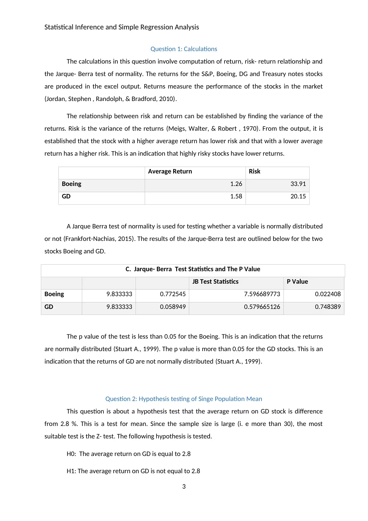
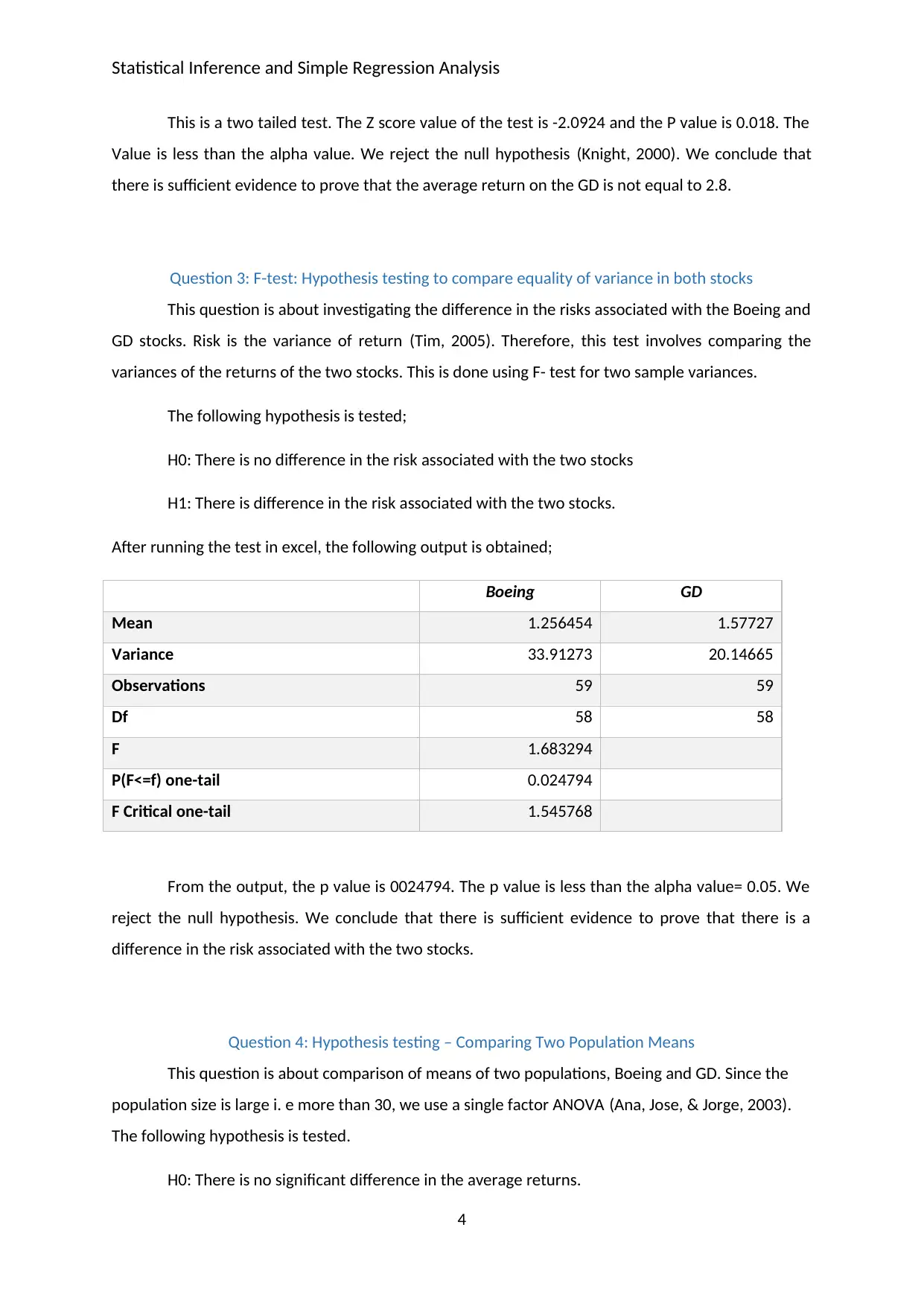
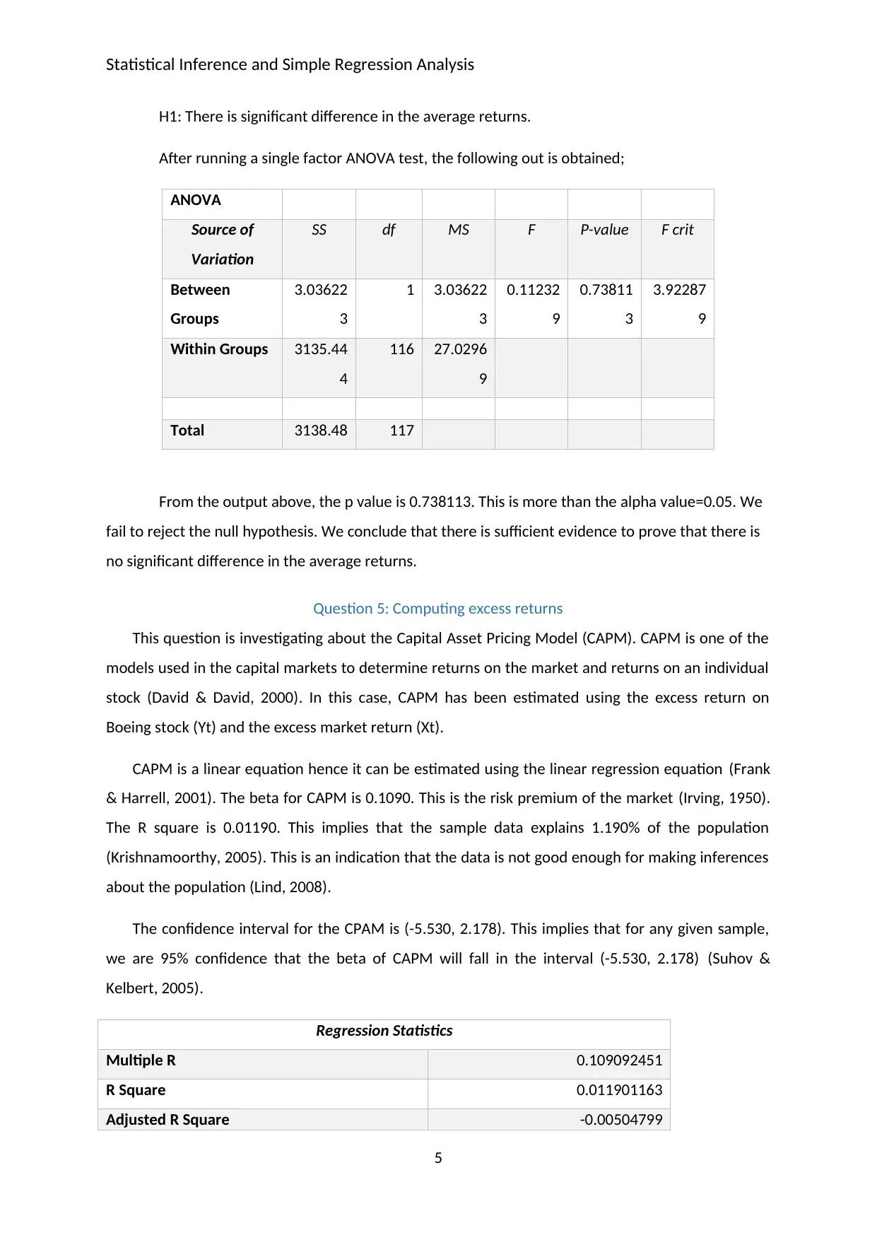
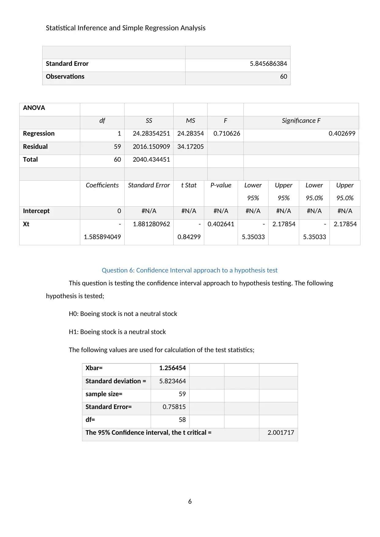
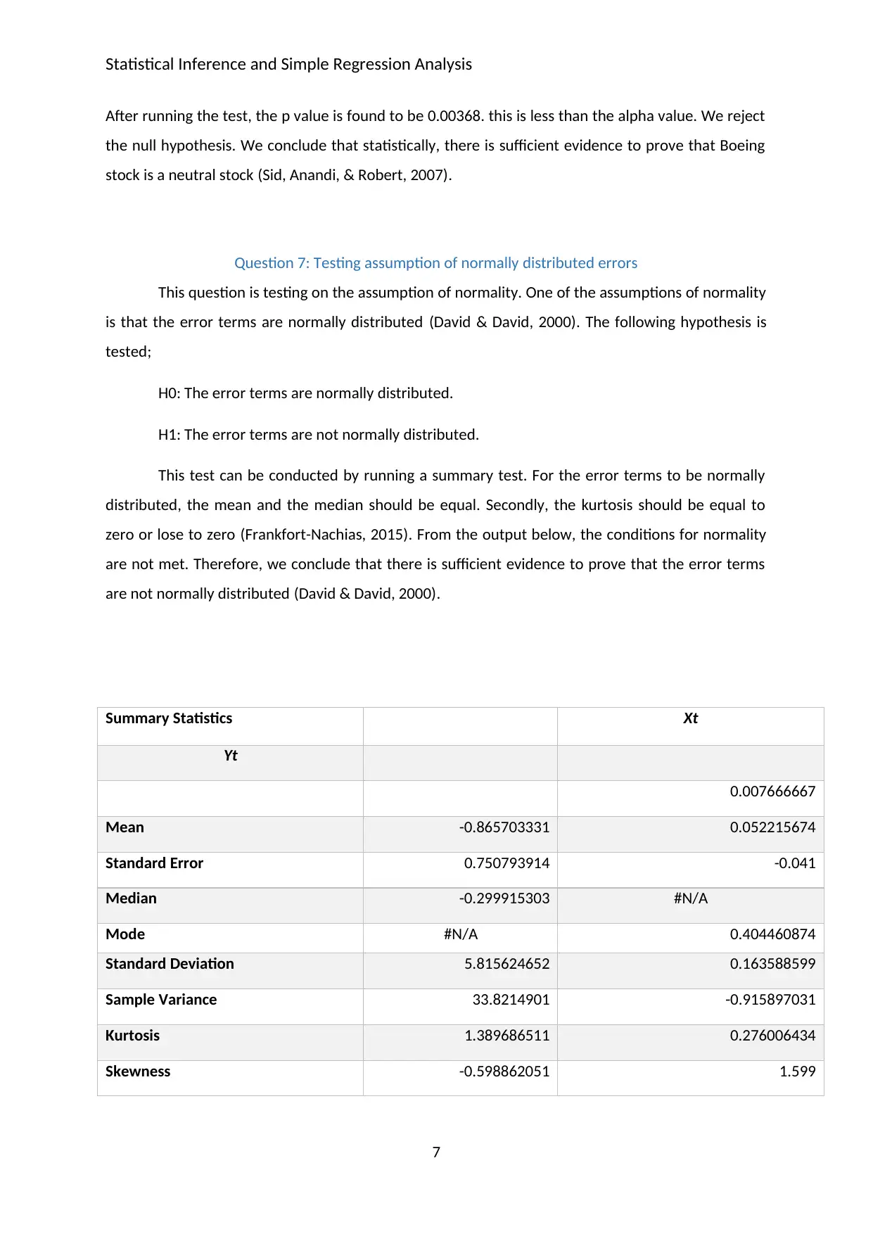
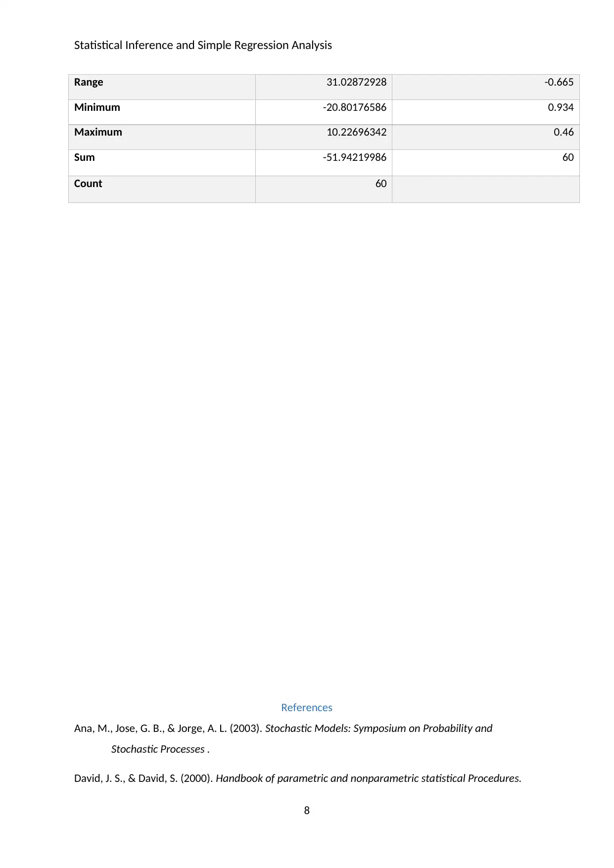
This assignment report provides a comprehensive analysis of statistical inference and simple regression techniques applied to financial data. It begins with calculations of returns, risk, and the Jarque-Bera test for normality on stock data. The report then delves into hypothesis testing for single population means, variance comparisons using the F-test, and comparing two population means using ANOVA. The Capital Asset Pricing Model (CAPM) is explored through regression analysis, including the interpretation of beta, R-squared, and confidence intervals. Additionally, the assignment covers the confidence interval approach to hypothesis testing and tests the assumption of normally distributed errors. The report provides detailed outputs, interpretations, and conclusions for each statistical test, demonstrating a solid understanding of the concepts and their practical application in finance.

Running head: STATISTICS 1
Institution
Business Statistics
Student Name
Student Id
Assignment 2: Statistical Inference and Simple Regression Analysis

Statistical Inference and Simple Regression Analysis
Contents
Question 1: Calculations........................................................................................................................2
Question 2: Hypothesis testing of Singe Population Mean....................................................................3
Question 3: F-test: Hypothesis testing to compare equality of variance in both stocks........................3
Question 4: Hypothesis testing – Comparing Two Population Means...................................................4
Question 5: Computing excess returns..................................................................................................4
Question 6: Confidence Interval approach to a hypothesis test............................................................5
Question 7: Testing assumption of normally distributed errors............................................................6
References.............................................................................................................................................8
2

Statistical Inference and Simple Regression Analysis
Question 1: Calculations
The calculations in this question involve computation of return, risk- return relationship and
the Jarque- Berra test of normality. The returns for the S&P, Boeing, DG and Treasury notes stocks
are produced in the excel output. Returns measure the performance of the stocks in the market
(Jordan, Stephen , Randolph, & Bradford, 2010).
The relationship between risk and return can be established by finding the variance of the
returns. Risk is the variance of the returns (Meigs, Walter, & Robert , 1970). From the output, it is
established that the stock with a higher average return has lower risk and that with a lower average
return has a higher risk. This is an indication that highly risky stocks have lower returns.
Average Return Risk
Boeing 1.26 33.91
GD 1.58 20.15
A Jarque Berra test of normality is used for testing whether a variable is normally distributed
or not (Frankfort-Nachias, 2015). The results of the Jarque-Berra test are outlined below for the two
stocks Boeing and GD.
C. Jarque- Berra Test Statistics and The P Value
JB Test Statistics P Value
Boeing 9.833333 0.772545 7.596689773 0.022408
GD 9.833333 0.058949 0.579665126 0.748389
The p value of the test is less than 0.05 for the Boeing. This is an indication that the returns
are normally distributed (Stuart A., 1999). The p value is more than 0.05 for the GD stocks. This is an
indication that the returns of GD are not normally distributed (Stuart A., 1999).
Question 2: Hypothesis testing of Singe Population Mean
This question is about a hypothesis test that the average return on GD stock is difference
from 2.8 %. This is a test for mean. Since the sample size is large (i. e more than 30), the most
suitable test is the Z- test. The following hypothesis is tested.
H0: The average return on GD is equal to 2.8
H1: The average return on GD is not equal to 2.8
3

Statistical Inference and Simple Regression Analysis
This is a two tailed test. The Z score value of the test is -2.0924 and the P value is 0.018. The
Value is less than the alpha value. We reject the null hypothesis (Knight, 2000). We conclude that
there is sufficient evidence to prove that the average return on the GD is not equal to 2.8.
Question 3: F-test: Hypothesis testing to compare equality of variance in both stocks
This question is about investigating the difference in the risks associated with the Boeing and
GD stocks. Risk is the variance of return (Tim, 2005). Therefore, this test involves comparing the
variances of the returns of the two stocks. This is done using F- test for two sample variances.
The following hypothesis is tested;
H0: There is no difference in the risk associated with the two stocks
H1: There is difference in the risk associated with the two stocks.
After running the test in excel, the following output is obtained;
Boeing GD
Mean 1.256454 1.57727
Variance 33.91273 20.14665
Observations 59 59
Df 58 58
F 1.683294
P(F<=f) one-tail 0.024794
F Critical one-tail 1.545768
From the output, the p value is 0024794. The p value is less than the alpha value= 0.05. We
reject the null hypothesis. We conclude that there is sufficient evidence to prove that there is a
difference in the risk associated with the two stocks.
Question 4: Hypothesis testing – Comparing Two Population Means
This question is about comparison of means of two populations, Boeing and GD. Since the
population size is large i. e more than 30, we use a single factor ANOVA (Ana, Jose, & Jorge, 2003).
The following hypothesis is tested.
H0: There is no significant difference in the average returns.
4

Statistical Inference and Simple Regression Analysis
H1: There is significant difference in the average returns.
After running a single factor ANOVA test, the following out is obtained;
ANOVA
Source of
Variation
SS df MS F P-value F crit
Between
Groups
3.03622
3
1 3.03622
3
0.11232
9
0.73811
3
3.92287
9
Within Groups 3135.44
4
116 27.0296
9
Total 3138.48 117
From the output above, the p value is 0.738113. This is more than the alpha value=0.05. We
fail to reject the null hypothesis. We conclude that there is sufficient evidence to prove that there is
no significant difference in the average returns.
Question 5: Computing excess returns
This question is investigating about the Capital Asset Pricing Model (CAPM). CAPM is one of the
models used in the capital markets to determine returns on the market and returns on an individual
stock (David & David, 2000). In this case, CAPM has been estimated using the excess return on
Boeing stock (Yt) and the excess market return (Xt).
CAPM is a linear equation hence it can be estimated using the linear regression equation (Frank
& Harrell, 2001). The beta for CAPM is 0.1090. This is the risk premium of the market (Irving, 1950).
The R square is 0.01190. This implies that the sample data explains 1.190% of the population
(Krishnamoorthy, 2005). This is an indication that the data is not good enough for making inferences
about the population (Lind, 2008).
The confidence interval for the CPAM is (-5.530, 2.178). This implies that for any given sample,
we are 95% confidence that the beta of CAPM will fall in the interval (-5.530, 2.178) (Suhov &
Kelbert, 2005).
Regression Statistics
Multiple R 0.109092451
R Square 0.011901163
Adjusted R Square -0.00504799
5

Statistical Inference and Simple Regression Analysis
Standard Error 5.845686384
Observations 60
ANOVA
df SS MS F Significance F
Regression 1 24.28354251 24.28354 0.710626 0.402699
Residual 59 2016.150909 34.17205
Total 60 2040.434451
Coefficients Standard Error t Stat P-value Lower
95%
Upper
95%
Lower
95.0%
Upper
95.0%
Intercept 0 #N/A #N/A #N/A #N/A #N/A #N/A #N/A
Xt -
1.585894049
1.881280962 -
0.84299
0.402641 -
5.35033
2.17854 -
5.35033
2.17854
Question 6: Confidence Interval approach to a hypothesis test
This question is testing the confidence interval approach to hypothesis testing. The following
hypothesis is tested;
H0: Boeing stock is not a neutral stock
H1: Boeing stock is a neutral stock
The following values are used for calculation of the test statistics;
Xbar= 1.256454
Standard deviation = 5.823464
sample size= 59
Standard Error= 0.75815
df= 58
The 95% Confidence interval, the t critical = 2.001717
6

Statistical Inference and Simple Regression Analysis
After running the test, the p value is found to be 0.00368. this is less than the alpha value. We reject
the null hypothesis. We conclude that statistically, there is sufficient evidence to prove that Boeing
stock is a neutral stock (Sid, Anandi, & Robert, 2007).
Question 7: Testing assumption of normally distributed errors
This question is testing on the assumption of normality. One of the assumptions of normality
is that the error terms are normally distributed (David & David, 2000). The following hypothesis is
tested;
H0: The error terms are normally distributed.
H1: The error terms are not normally distributed.
This test can be conducted by running a summary test. For the error terms to be normally
distributed, the mean and the median should be equal. Secondly, the kurtosis should be equal to
zero or lose to zero (Frankfort-Nachias, 2015). From the output below, the conditions for normality
are not met. Therefore, we conclude that there is sufficient evidence to prove that the error terms
are not normally distributed (David & David, 2000).
Summary Statistics Xt
Yt
0.007666667
Mean -0.865703331 0.052215674
Standard Error 0.750793914 -0.041
Median -0.299915303 #N/A
Mode #N/A 0.404460874
Standard Deviation 5.815624652 0.163588599
Sample Variance 33.8214901 -0.915897031
Kurtosis 1.389686511 0.276006434
Skewness -0.598862051 1.599
7

Statistical Inference and Simple Regression Analysis
Range 31.02872928 -0.665
Minimum -20.80176586 0.934
Maximum 10.22696342 0.46
Sum -51.94219986 60
Count 60
References
Ana, M., Jose, G. B., & Jorge, A. L. (2003). Stochastic Models: Symposium on Probability and
Stochastic Processes .
David, J. S., & David, S. (2000). Handbook of parametric and nonparametric statistical Procedures.
8

Statistical Inference and Simple Regression Analysis
Frank, E., & Harrell, J. (2001). Regression Modelling Strategies: Models, Logistic Regression, and
Survival Analysis.
Frankfort-Nachias, C. &.-G. (2015). Social Statistics for a diverse society. Thousand Oaks, CA: Sage
Publications.
Irving, J. G. (1950). Probability and the Weighing Evidence.
Jordan, Stephen , A. R., Randolph, W. W., & Bradford, D. (2010). Fundamentals of corporate finance.
Boston: McGraw-Hill Irwin.
Knight, K. (2000). Mathematical Statistics- Volume in Texts in Statistical Scence Series. Chapman and
Hall.
Krishnamoorthy, K. (2005). Handbook of Statistical Distributions with Applications.
Lind, D. A. (2008). Statistical Techniques in Business & . Boston.: McGraw-Hill Irwin.
Meigs, Walter, B., & Robert , F. (1970). Financial Accounting. McGraw-Hill Book Company.
Sid, M., Anandi, P. S., & Robert, A. C. (2007). Practicing Financial Planning for Proffesionals .
Rochester Hills Publishing.
Stuart A., O. K. (1999). Kendall’s Advanced Theory of Statistics: Volume 2A- Classical Inference & the
linear Model.
Suhov, Y., & Kelbert, M. (2005). Probability and Statisics by exasmple. basic probability and statistics.
Tim, S. (2005). Mastering Statistical Process Control: A handbook for Performance Improvement
Using Cases.
9