Statistical Analysis of Income and Turnover: A Management Report
VerifiedAdded on 2020/06/05
|19
|2556
|227
Report
AI Summary
This report presents a statistical analysis of various aspects of business and economics. It begins by examining changes in gross annual earnings in the public and private sectors since 2009, including an assessment of the gender pay gap. The report then delves into hourly earnings data, calculating descriptive statistics like mean and standard deviation and comparing results across different geographic areas. Regression analysis is employed to study the relationship between floor area and weekly turnover, determining the correlation coefficient, calculating turnover based on floor size, and assessing the statistical validity of the model. Furthermore, the report analyzes delivery numbers, economic order quantity (EOQ), and associated costs to optimize inventory management. The analysis includes scatter diagrams to visualize relationships between variables and detailed interpretations of the findings, supported by tables, figures, and relevant statistical formulas.

STATISTICS FOR MANAGEMENT
Paraphrase This Document
Need a fresh take? Get an instant paraphrase of this document with our AI Paraphraser
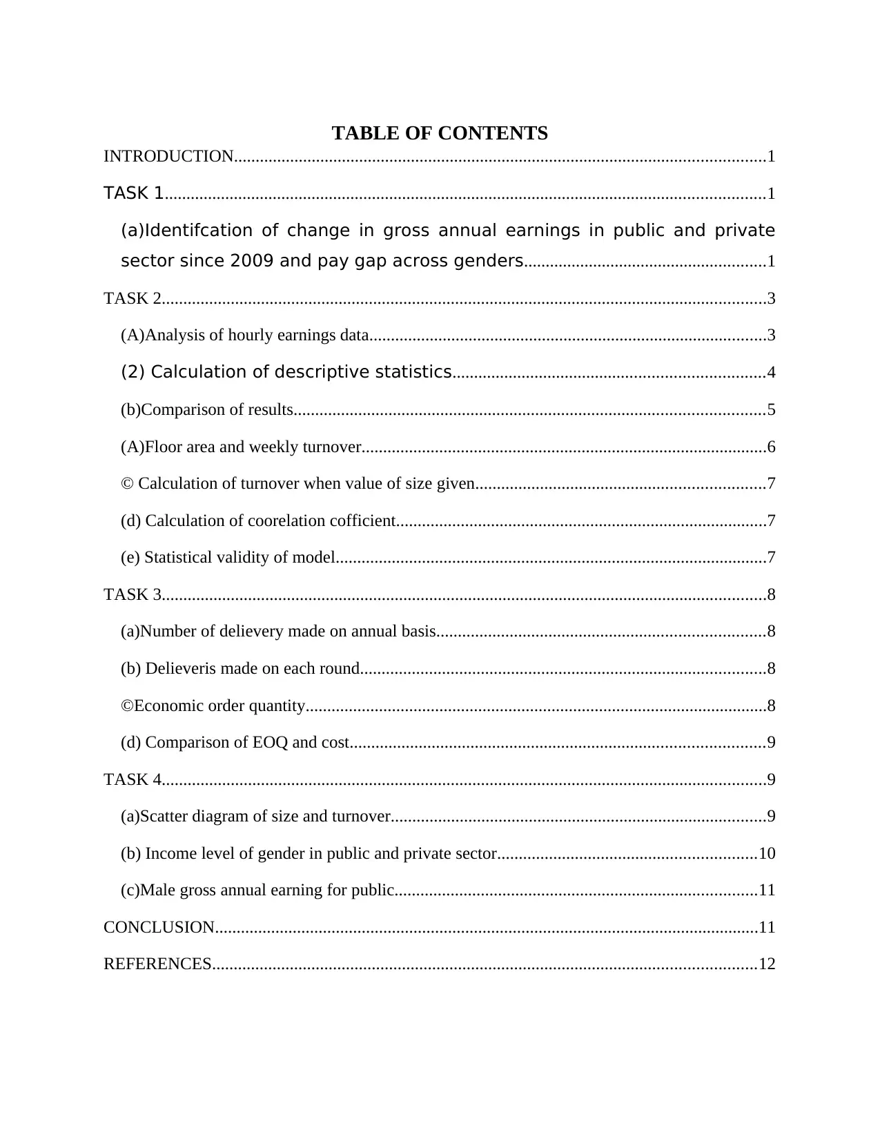
TABLE OF CONTENTS
INTRODUCTION...........................................................................................................................1
TASK 1...........................................................................................................................................1
(a)Identifcation of change in gross annual earnings in public and private
sector since 2009 and pay gap across genders........................................................1
TASK 2............................................................................................................................................3
(A)Analysis of hourly earnings data............................................................................................3
(2) Calculation of descriptive statistics........................................................................4
(b)Comparison of results.............................................................................................................5
(A)Floor area and weekly turnover..............................................................................................6
© Calculation of turnover when value of size given...................................................................7
(d) Calculation of coorelation cofficient......................................................................................7
(e) Statistical validity of model....................................................................................................7
TASK 3............................................................................................................................................8
(a)Number of delievery made on annual basis............................................................................8
(b) Delieveris made on each round..............................................................................................8
©Economic order quantity...........................................................................................................8
(d) Comparison of EOQ and cost................................................................................................9
TASK 4............................................................................................................................................9
(a)Scatter diagram of size and turnover.......................................................................................9
(b) Income level of gender in public and private sector............................................................10
(c)Male gross annual earning for public....................................................................................11
CONCLUSION..............................................................................................................................11
REFERENCES..............................................................................................................................12
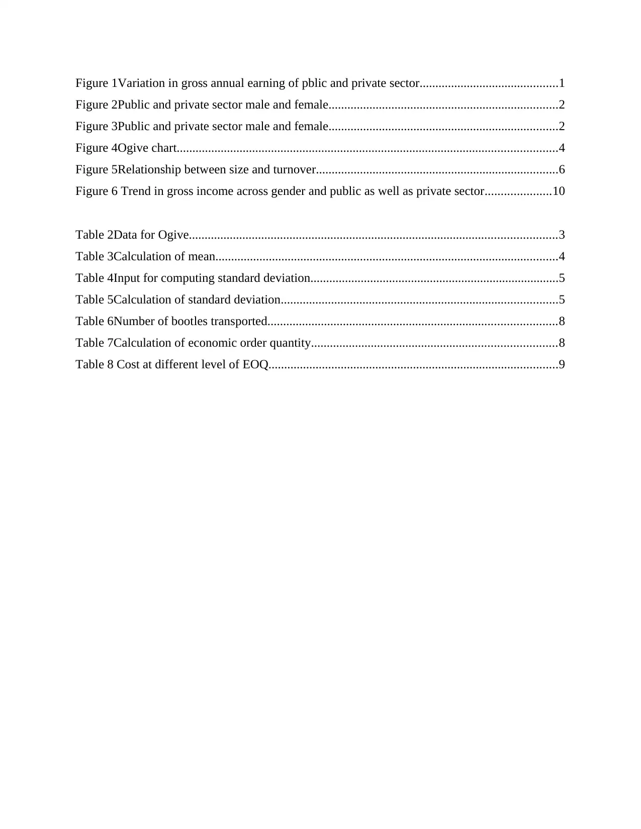
Figure 1Variation in gross annual earning of pblic and private sector............................................1
Figure 2Public and private sector male and female.........................................................................2
Figure 3Public and private sector male and female.........................................................................2
Figure 4Ogive chart.........................................................................................................................4
Figure 5Relationship between size and turnover.............................................................................6
Figure 6 Trend in gross income across gender and public as well as private sector.....................10
Table 2Data for Ogive.....................................................................................................................3
Table 3Calculation of mean.............................................................................................................4
Table 4Input for computing standard deviation...............................................................................5
Table 5Calculation of standard deviation........................................................................................5
Table 6Number of bootles transported............................................................................................8
Table 7Calculation of economic order quantity..............................................................................8
Table 8 Cost at different level of EOQ............................................................................................9
⊘ This is a preview!⊘
Do you want full access?
Subscribe today to unlock all pages.
Trusted by 1+ million students worldwide
INTRODUCTION
Statistics is widely used to understand data and identifying hidden trends. There are
number of tools and techniques that can be used to analyze data deeply and in proper manner. In
current report data related to income level of male and female in public and private sector is
analyzed. Apart from this, by using regression analysis method relationship between dependent
and independent variable is identified and validity of model is determined. At end of the report
through graphical representations analysis is done and in this way entire work is carried out.
TASK 1
(a)Identifcation of change in gross annual earnings in public and private
sector since 2009 and pay gap across genders
Figure1 Variation in gross annual earning of pblic and private sector
Interpretation
Gross annual income in public sector was 3% in year 2010 and same
was -1% in case of private sector. Thus, in this year annual earnings
increased in public sector and same reduced in comparison to previous year.
Percentage change in public and private sector almost remain same and in
year 2016, annual earning just increase by 1% and while it increased by 3%
in case of private sector. Hence, it can be said that income in private sector
is increasing at rapid rate then public sector.
1 | P a g e
Paraphrase This Document
Need a fresh take? Get an instant paraphrase of this document with our AI Paraphraser
2009 2010 2011 2012 2013 2014 2015
0
5000
10000
15000
20000
25000
30000
35000
40000
30638 31264 31380 31816 32541 32878 33685
27362 27000 27233 27705 28201 28442 28881
25224 26113 26470 26636 27338 27705 27900
19551 19532 19565 20313 20698 21017 21403
Chart Title
Public sector male Private sector male
Public sector female Private sector female
Figure2 Public and private sector male and female
2009 2010 2011 2012 2013 2014 2015
0
5000
10000
15000
20000
25000
30000
35000
40000
Chart Title
Public sector male Private sector male
Public sector female Private sector female
Figure3 Public and private sector male and female
2 | P a g e
0
5000
10000
15000
20000
25000
30000
35000
40000
30638 31264 31380 31816 32541 32878 33685
27362 27000 27233 27705 28201 28442 28881
25224 26113 26470 26636 27338 27705 27900
19551 19532 19565 20313 20698 21017 21403
Chart Title
Public sector male Private sector male
Public sector female Private sector female
Figure2 Public and private sector male and female
2009 2010 2011 2012 2013 2014 2015
0
5000
10000
15000
20000
25000
30000
35000
40000
Chart Title
Public sector male Private sector male
Public sector female Private sector female
Figure3 Public and private sector male and female
2 | P a g e
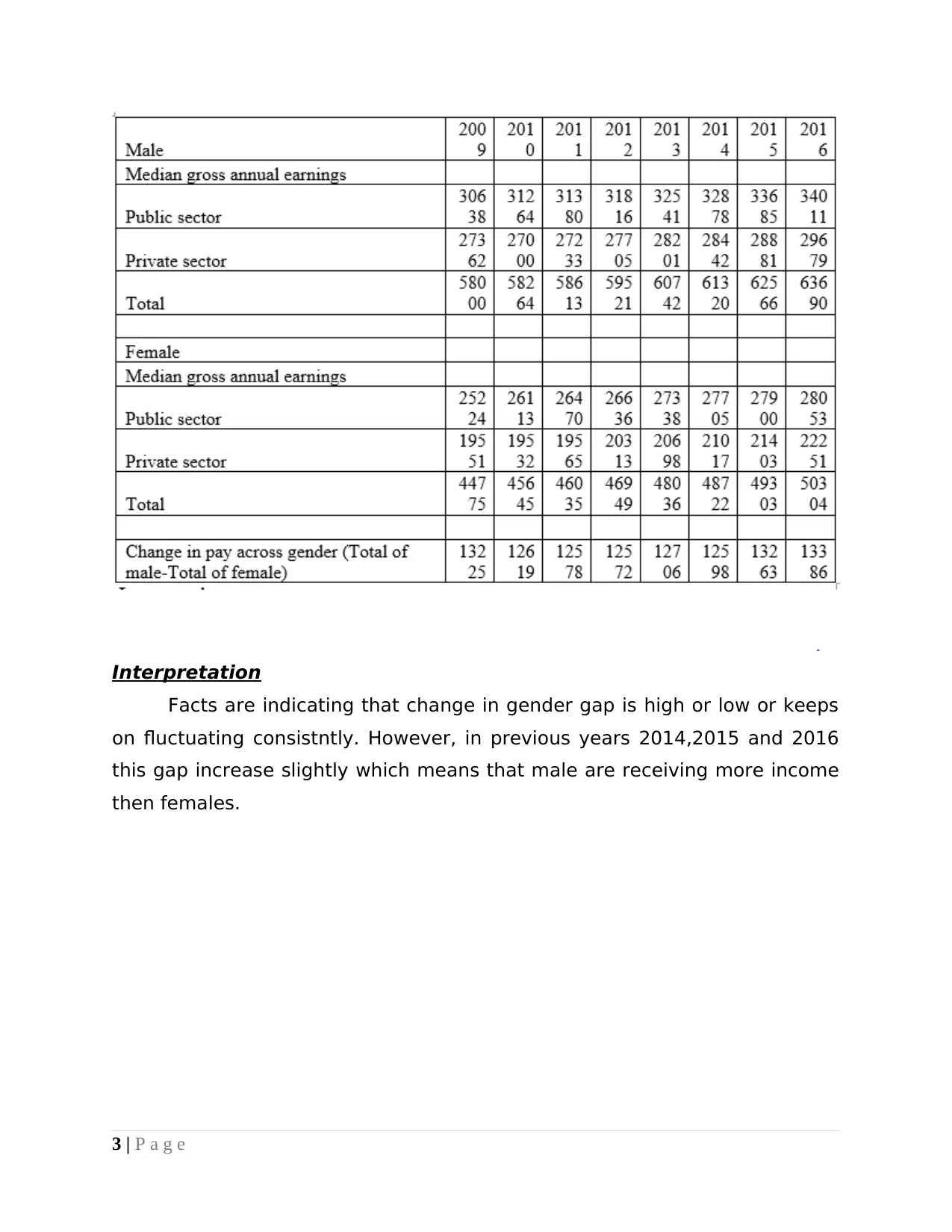
Interpretation
Facts are indicating that change in gender gap is high or low or keeps
on fluctuating consistntly. However, in previous years 2014,2015 and 2016
this gap increase slightly which means that male are receiving more income
then females.
3 | P a g e
Facts are indicating that change in gender gap is high or low or keeps
on fluctuating consistntly. However, in previous years 2014,2015 and 2016
this gap increase slightly which means that male are receiving more income
then females.
3 | P a g e
⊘ This is a preview!⊘
Do you want full access?
Subscribe today to unlock all pages.
Trusted by 1+ million students worldwide
2009 2010 2011 2012 2013 2014 2015 2016
0
5000
10000
15000
20000
25000
30000
35000
40000
30638 31264313803181632541 328783368534011
27362 27000272332770528201 284422888129679
Public sector male
Private sector male
Figure 4Public and private sector male income level
2009 2010 2011 2012 2013 2014 2015 2016
0
10000
20000
30000
40000
50000
60000
70000
2522426113264702663627338277052790028053
19551195321956520313206982101721403
63690
Public sector female
Private sector female
Figure 5Public and private sector female income level
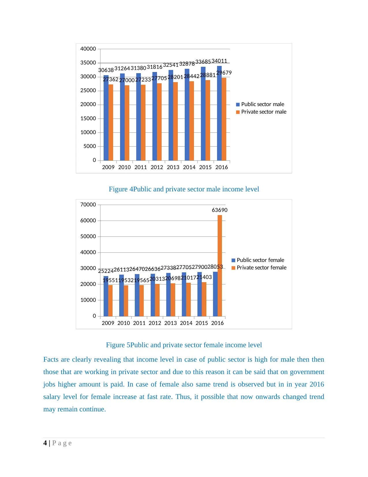
Facts are clearly revealing that income level in case of public sector is high for male then then
those that are working in private sector and due to this reason it can be said that on government
jobs higher amount is paid. In case of female also same trend is observed but in in year 2016
salary level for female increase at fast rate. Thus, it possible that now onwards changed trend
may remain continue.
4 | P a g e
0
5000
10000
15000
20000
25000
30000
35000
40000
30638 31264313803181632541 328783368534011
27362 27000272332770528201 284422888129679
Public sector male
Private sector male
Figure 4Public and private sector male income level
2009 2010 2011 2012 2013 2014 2015 2016
0
10000
20000
30000
40000
50000
60000
70000
2522426113264702663627338277052790028053
19551195321956520313206982101721403
63690
Public sector female
Private sector female
Figure 5Public and private sector female income level
Facts are clearly revealing that income level in case of public sector is high for male then then
those that are working in private sector and due to this reason it can be said that on government
jobs higher amount is paid. In case of female also same trend is observed but in in year 2016
salary level for female increase at fast rate. Thus, it possible that now onwards changed trend
may remain continue.
4 | P a g e
Paraphrase This Document
Need a fresh take? Get an instant paraphrase of this document with our AI Paraphraser
TASK 2
(A)Analysis of hourly earnings data
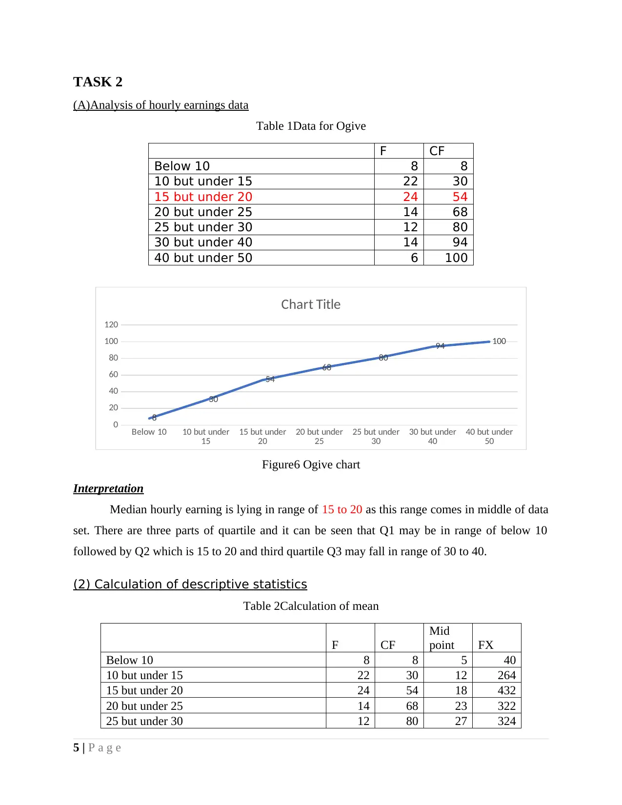
Table 1Data for Ogive
F CF
Below 10 8 8
10 but under 15 22 30
15 but under 20 24 54
20 but under 25 14 68
25 but under 30 12 80
30 but under 40 14 94
40 but under 50 6 100
Below 10 10 but under
15 15 but under
20 20 but under
25 25 but under
30 30 but under
40 40 but under
50
0
20
40
60
80
100
120
8
30
54
68
80
94 100
Chart Title
Figure6 Ogive chart
Interpretation
Median hourly earning is lying in range of 15 to 20 as this range comes in middle of data
set. There are three parts of quartile and it can be seen that Q1 may be in range of below 10
followed by Q2 which is 15 to 20 and third quartile Q3 may fall in range of 30 to 40.
(2) Calculation of descriptive statistics
Table 2Calculation of mean
F CF
Mid
point FX
Below 10 8 8 5 40
10 but under 15 22 30 12 264
15 but under 20 24 54 18 432
20 but under 25 14 68 23 322
25 but under 30 12 80 27 324
5 | P a g e
(A)Analysis of hourly earnings data
Table 1Data for Ogive
F CF
Below 10 8 8
10 but under 15 22 30
15 but under 20 24 54
20 but under 25 14 68
25 but under 30 12 80
30 but under 40 14 94
40 but under 50 6 100
Below 10 10 but under
15 15 but under
20 20 but under
25 25 but under
30 30 but under
40 40 but under
50
0
20
40
60
80
100
120
8
30
54
68
80
94 100
Chart Title
Figure6 Ogive chart
Interpretation
Median hourly earning is lying in range of 15 to 20 as this range comes in middle of data
set. There are three parts of quartile and it can be seen that Q1 may be in range of below 10
followed by Q2 which is 15 to 20 and third quartile Q3 may fall in range of 30 to 40.
(2) Calculation of descriptive statistics
Table 2Calculation of mean
F CF
Mid
point FX
Below 10 8 8 5 40
10 but under 15 22 30 12 264
15 but under 20 24 54 18 432
20 but under 25 14 68 23 322
25 but under 30 12 80 27 324
5 | P a g e
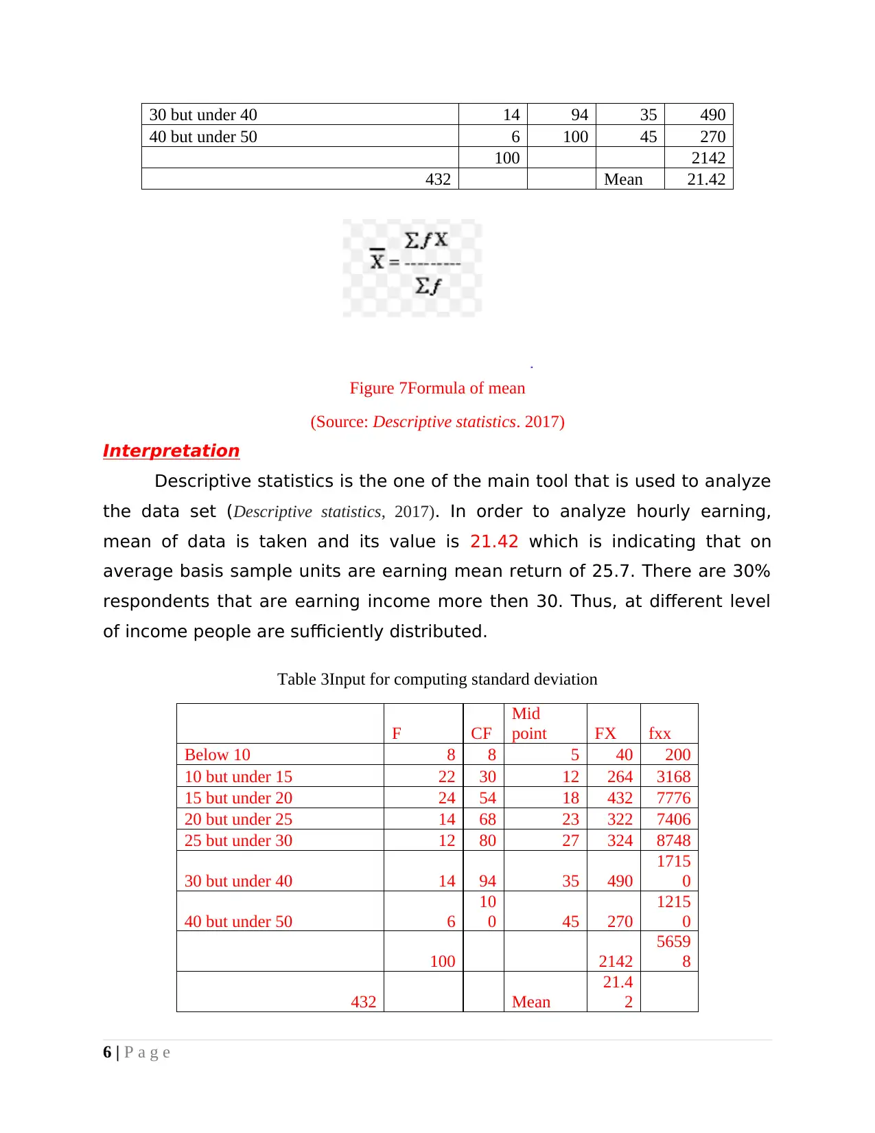
30 but under 40 14 94 35 490
40 but under 50 6 100 45 270
100 2142
432 Mean 21.42
Figure 7Formula of mean
(Source: Descriptive statistics. 2017)
Interpretation
Descriptive statistics is the one of the main tool that is used to analyze
the data set (Descriptive statistics, 2017). In order to analyze hourly earning,
mean of data is taken and its value is 21.42 which is indicating that on
average basis sample units are earning mean return of 25.7. There are 30%
respondents that are earning income more then 30. Thus, at different level
of income people are sufficiently distributed.
Table 3Input for computing standard deviation
F CF
Mid
point FX fxx
Below 10 8 8 5 40 200
10 but under 15 22 30 12 264 3168
15 but under 20 24 54 18 432 7776
20 but under 25 14 68 23 322 7406
25 but under 30 12 80 27 324 8748
30 but under 40 14 94 35 490
1715
0
40 but under 50 6
10
0 45 270
1215
0
100 2142
5659
8
432 Mean
21.4
2
6 | P a g e
⊘ This is a preview!⊘
Do you want full access?
Subscribe today to unlock all pages.
Trusted by 1+ million students worldwide
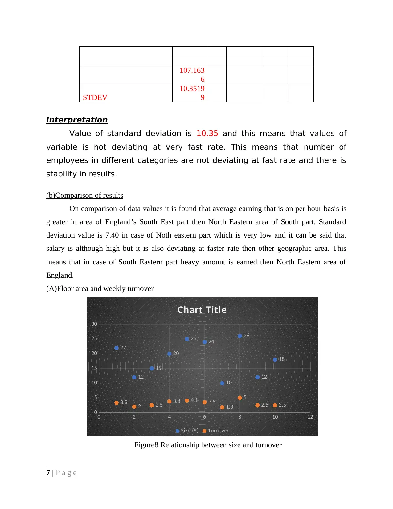
107.163
6
STDEV
10.3519
9
Interpretation
Value of standard deviation is 10.35 and this means that values of
variable is not deviating at very fast rate. This means that number of
employees in different categories are not deviating at fast rate and there is
stability in results.
(b)Comparison of results
On comparison of data values it is found that average earning that is on per hour basis is
greater in area of England’s South East part then North Eastern area of South part. Standard
deviation value is 7.40 in case of Noth eastern part which is very low and it can be said that
salary is although high but it is also deviating at faster rate then other geographic area. This
means that in case of South Eastern part heavy amount is earned then North Eastern area of
England.
(A)Floor area and weekly turnover
0 2 4 6 8 10 12
0
5
10
15
20
25
30
3.3 2 2.5 3.8 4.1 3.5 1.8
5
2.5 2.5
22
12
15
20
25 24
10
26
12
18
Chart Title
Size (S) Turnover
Figure8 Relationship between size and turnover
7 | P a g e
Paraphrase This Document
Need a fresh take? Get an instant paraphrase of this document with our AI Paraphraser
0 2 4 6 8 10 12
0
2
4
6
8
10
12
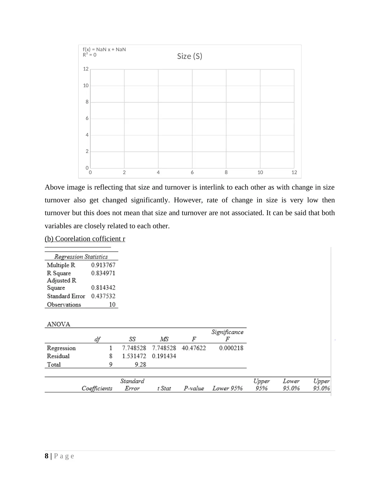
f(x) = NaN x + NaN
R² = 0 Size (S)
Above image is reflecting that size and turnover is interlink to each other as with change in size
turnover also get changed significantly. However, rate of change in size is very low then
turnover but this does not mean that size and turnover are not associated. It can be said that both
variables are closely related to each other.
(b) Coorelation cofficient r
8 | P a g e
0
2
4
6
8
10
12
f(x) = NaN x + NaN
R² = 0 Size (S)
Above image is reflecting that size and turnover is interlink to each other as with change in size
turnover also get changed significantly. However, rate of change in size is very low then
turnover but this does not mean that size and turnover are not associated. It can be said that both
variables are closely related to each other.
(b) Coorelation cofficient r
8 | P a g e
1.5 2 2.5 3 3.5 4 4.5 5 5.5
0
5
10
15
20
25
30
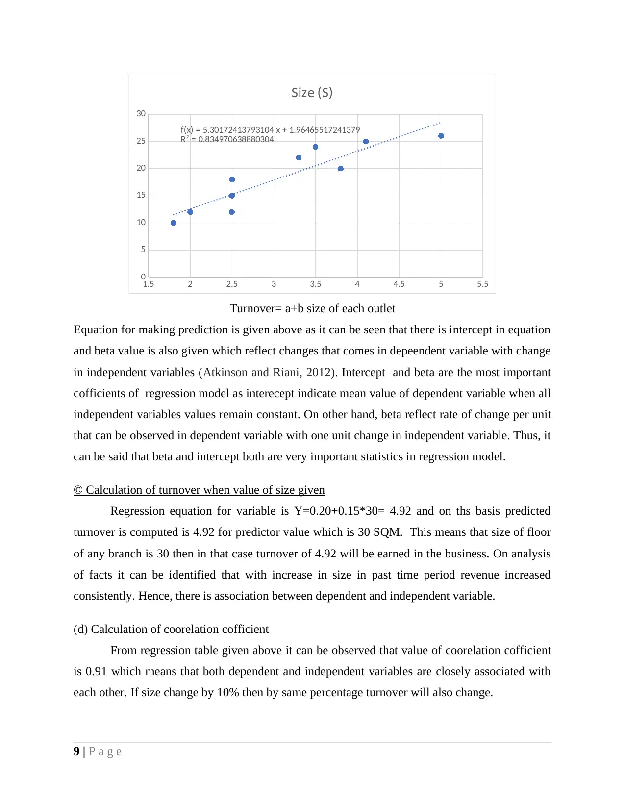
f(x) = 5.30172413793104 x + 1.96465517241379
R² = 0.834970638880304
Size (S)
Turnover= a+b size of each outlet
Equation for making prediction is given above as it can be seen that there is intercept in equation
and beta value is also given which reflect changes that comes in depeendent variable with change
in independent variables (Atkinson and Riani, 2012). Intercept and beta are the most important
cofficients of regression model as interecept indicate mean value of dependent variable when all
independent variables values remain constant. On other hand, beta reflect rate of change per unit
that can be observed in dependent variable with one unit change in independent variable. Thus, it
can be said that beta and intercept both are very important statistics in regression model.
© Calculation of turnover when value of size given
Regression equation for variable is Y=0.20+0.15*30= 4.92 and on ths basis predicted
turnover is computed is 4.92 for predictor value which is 30 SQM. This means that size of floor
of any branch is 30 then in that case turnover of 4.92 will be earned in the business. On analysis
of facts it can be identified that with increase in size in past time period revenue increased
consistently. Hence, there is association between dependent and independent variable.
(d) Calculation of coorelation cofficient
From regression table given above it can be observed that value of coorelation cofficient
is 0.91 which means that both dependent and independent variables are closely associated with
each other. If size change by 10% then by same percentage turnover will also change.
9 | P a g e
0
5
10
15
20
25
30
f(x) = 5.30172413793104 x + 1.96465517241379
R² = 0.834970638880304
Size (S)
Turnover= a+b size of each outlet
Equation for making prediction is given above as it can be seen that there is intercept in equation
and beta value is also given which reflect changes that comes in depeendent variable with change
in independent variables (Atkinson and Riani, 2012). Intercept and beta are the most important
cofficients of regression model as interecept indicate mean value of dependent variable when all
independent variables values remain constant. On other hand, beta reflect rate of change per unit
that can be observed in dependent variable with one unit change in independent variable. Thus, it
can be said that beta and intercept both are very important statistics in regression model.
© Calculation of turnover when value of size given
Regression equation for variable is Y=0.20+0.15*30= 4.92 and on ths basis predicted
turnover is computed is 4.92 for predictor value which is 30 SQM. This means that size of floor
of any branch is 30 then in that case turnover of 4.92 will be earned in the business. On analysis
of facts it can be identified that with increase in size in past time period revenue increased
consistently. Hence, there is association between dependent and independent variable.
(d) Calculation of coorelation cofficient
From regression table given above it can be observed that value of coorelation cofficient
is 0.91 which means that both dependent and independent variables are closely associated with
each other. If size change by 10% then by same percentage turnover will also change.
9 | P a g e
⊘ This is a preview!⊘
Do you want full access?
Subscribe today to unlock all pages.
Trusted by 1+ million students worldwide
1 out of 19
Related Documents


Your All-in-One AI-Powered Toolkit for Academic Success.
+13062052269
info@desklib.com
Available 24*7 on WhatsApp / Email
![[object Object]](/_next/static/media/star-bottom.7253800d.svg)
Unlock your academic potential
Copyright © 2020–2026 A2Z Services. All Rights Reserved. Developed and managed by ZUCOL.