Analyzing Job Income and Employment Data Using SPSS Techniques

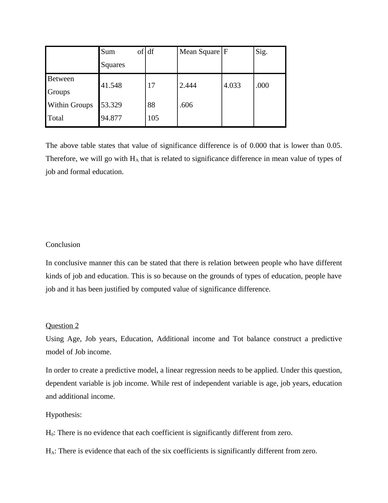
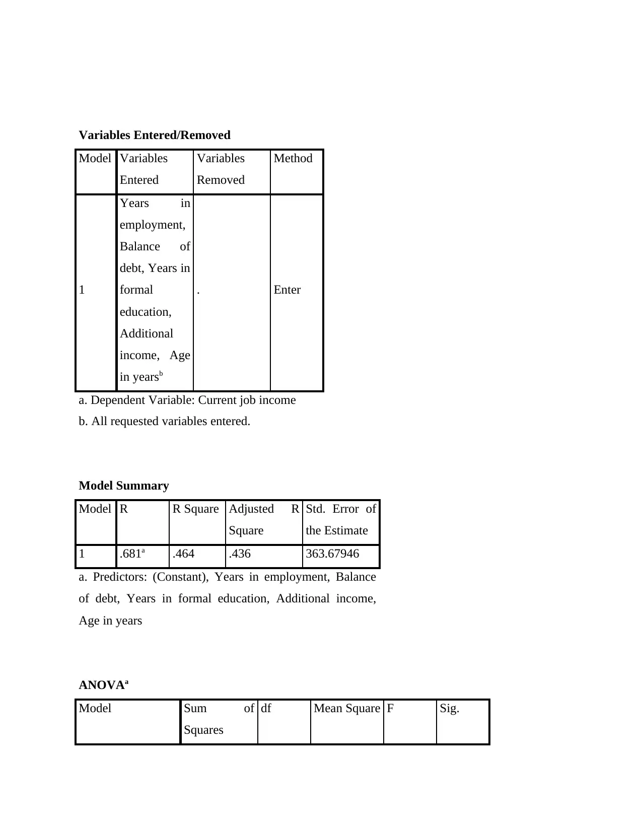
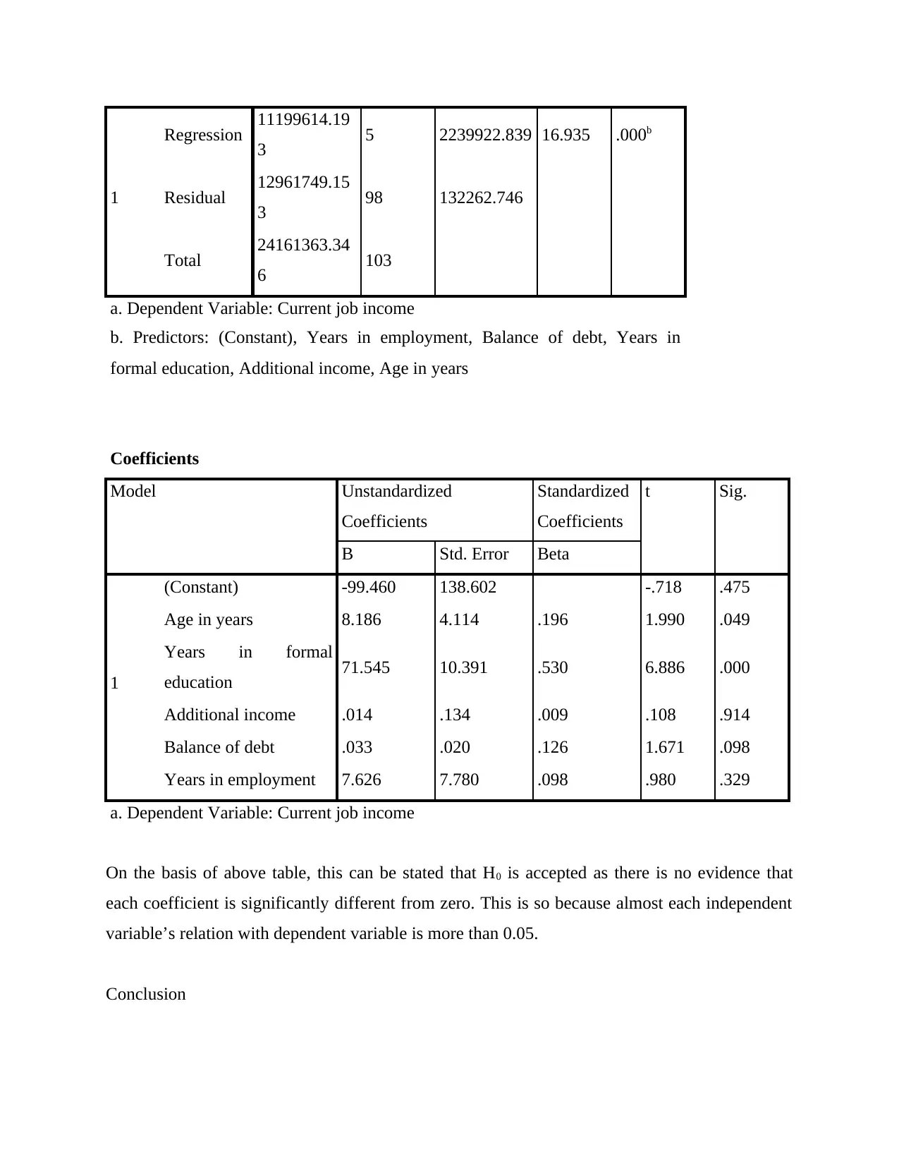
This assignment solution presents a comprehensive analysis of a dataset using SPSS, focusing on the relationships between job types, education, income, and gender. The analysis begins with an ANOVA test to determine the significance of differences in formal education among different job types, concluding that there is a statistically significant relationship. A linear regression model is then constructed to predict job income using variables like age, job years, education, and additional income. The regression analysis reveals that the null hypothesis is accepted, indicating no significant relationship between these independent variables and job income based on the provided data. Finally, an independent samples t-test is used to compare years in employment between male and female respondents, which supports the claim that years in employment are significantly lower for female respondents. The assignment demonstrates the application of various statistical techniques within SPSS to draw meaningful conclusions from the given dataset.

Assessment

Contents
INTRODUCTION.....................................................................................................................................3
Question 1...............................................................................................................................................3
Question 2...............................................................................................................................................4
Question 3...............................................................................................................................................7

INTRODUCTION
The given data set is based on local store who is planning whether they should issue a
credit or not. With an aim of finding a particular outcome, different kinds of SPSS tests have
been applied. The rationale behind applying such testes to assess significance difference between
formal education and job types. As well as descriptive analysis of given factors is also completed
under the project.
Question 1
The expectation is of significant difference in years in formal education (Education) between
types of jobs (Job type). Is this expectation supported by the data?
In the question, dependent data is related to types of job. In the given data set, types of job are
categorized in four segments which are as:
0.00 Manual
1.00 Unskilled
2.00 Skilled
3.00 Managerial
As question is asking to compare mean of dependent variable among different independent
variables regards to formal education.
Hypothesis:
H0: There is no significance difference in mean value of types of job and formal education.
HA: There is significance difference in mean value of types of job and formal education.
ANOVA
Type of job

Sum of
Squares
df Mean Square F Sig.
Between
Groups 41.548 17 2.444 4.033 .000
Within Groups 53.329 88 .606
Total 94.877 105
The above table states that value of significance difference is of 0.000 that is lower than 0.05.
Therefore, we will go with HA that is related to significance difference in mean value of types of
job and formal education.
Conclusion
In conclusive manner this can be stated that there is relation between people who have different
kinds of job and education. This is so because on the grounds of types of education, people have
job and it has been justified by computed value of significance difference.
Question 2
Using Age, Job years, Education, Additional income and Tot balance construct a predictive
model of Job income.
In order to create a predictive model, a linear regression needs to be applied. Under this question,
dependent variable is job income. While rest of independent variable is age, job years, education
and additional income.
Hypothesis:
H0: There is no evidence that each coefficient is significantly different from zero.
HA: There is evidence that each of the six coefficients is significantly different from zero.

Variables Entered/Removed
Model Variables
Entered
Variables
Removed
Method
1
Years in
employment,
Balance of
debt, Years in
formal
education,
Additional
income, Age
in yearsb
. Enter
a. Dependent Variable: Current job income
b. All requested variables entered.
Model Summary
Model R R Square Adjusted R
Square
Std. Error of
the Estimate
1 .681a .464 .436 363.67946
a. Predictors: (Constant), Years in employment, Balance
of debt, Years in formal education, Additional income,
Age in years
ANOVAa
Model Sum of
Squares
df Mean Square F Sig.

1
Regression 11199614.19
3 5 2239922.839 16.935 .000b
Residual 12961749.15
3 98 132262.746
Total 24161363.34
6 103
a. Dependent Variable: Current job income
b. Predictors: (Constant), Years in employment, Balance of debt, Years in
formal education, Additional income, Age in years
Coefficients
Model Unstandardized
Coefficients
Standardized
Coefficients
t Sig.
B Std. Error Beta
1
(Constant) -99.460 138.602 -.718 .475
Age in years 8.186 4.114 .196 1.990 .049
Years in formal
education 71.545 10.391 .530 6.886 .000
Additional income .014 .134 .009 .108 .914
Balance of debt .033 .020 .126 1.671 .098
Years in employment 7.626 7.780 .098 .980 .329
a. Dependent Variable: Current job income
On the basis of above table, this can be stated that H0 is accepted as there is no evidence that
each coefficient is significantly different from zero. This is so because almost each independent
variable’s relation with dependent variable is more than 0.05.
Conclusion

In terms of conclusion, it can be stated that current job income has no relation with different
kinds of factors like age, education, balance of debt etc. This is so because in ANOVA test, each
value of significant difference is greater than 0.05.
Question 3
Do the data support the claim that years in employment (Job years) is significantly lower for
female compared to male respondents (Gender)?
In this question, years in employment is considered as dependent variable. While another
variable is related to gender. In this aspect independent T test can be applied in such manner:
H0: There is no significant difference in variances in years in employment between female and
male.
HA: There is significant difference in variances in years in employment between female and
male.
α = level of significance 5% (0.05)
Group Statistics
Gender N Mean Std.
Deviation
Std. Error
Mean
Years in
employment
Female 24 1.5833 2.04124 .41667
Male 82 5.2439 6.75051 .74547
Independent Samples Test
Levene's
Test for
Equality of
Variances
t-test for Equality of Means

F Sig. t df Sig.
(2-
tailed
)
Mean
Differenc
e
Std.
Error
Differenc
e
95%
Confidence
Interval of the
Difference
Lower Upper
Years in
employme
nt
Equal
variance
s
assumed
10.78
2
.00
1
-
2.61
4
104 .010 -3.66057 1.40045
-
6.4377
2
-.8834
2
Equal
variance
s not
assumed
-
4.28
6
103.82
8 .000 -3.66057 .85401
-
5.3541
4
-
1.9670
0
On the basis of above table, this can be inferred that value of significance difference in Levene's
Test for Equality of Variances is of 0.001 that is lower than 0.05. Therefore, this can be
interpreted that H0 should be rejected as there is no significant difference in variances in years in
employment between female and male.
While in the t-test for Equality of Means the value of significance difference is more than 0.05.
Conclusion
As per the above table this can be concluded that level of significance difference is 0.001<0.05.
Thus we will retain to HA that is about existing significance difference in variances in years in
employment between female and male. And there is sufficient evidence that years in
employment (Job years) is significantly lower for female compared to male respondents
(Gender).