Statistical Analysis of Job Income and Credit Application (SPSS)

This report presents a comprehensive statistical analysis of job income and credit applications using SPSS software. The analysis includes descriptive statistics, such as mean, median, variance, skewness, and kurtosis, to understand the distribution of job income and identify outliers. Hypothesis testing, including t-tests and ANOVA, is employed to determine significant differences between groups, such as those who were granted credit versus those who were not, and to assess the impact of various factors on job income. The report also explores the assumptions underlying these statistical methods, such as normality, homoscedasticity, and independence of errors, and addresses how violations of these assumptions were handled. Furthermore, regression analysis is utilized to examine the relationship between job income and several independent variables, including class, sex, age, job years, education, marital status, management, and supervisory roles. The report concludes with a discussion of the findings and their implications, offering valuable insights into the factors influencing credit approval and income levels.

SPSS

TABLE OF CONTENTS
INTRODUCTION................................................................................................................................1
PART 1A..............................................................................................................................................1
1B.........................................................................................................................................................2
MEASUEMENT OF CENTRAL TENDANCY..................................................................................2
1C.........................................................................................................................................................4
ASSUMPTIONS..................................................................................................................................5
ONE WAY ANOVA............................................................................................................................5
Test of Homogeneity of Variances.......................................................................................................6
PART 2 REGRESSION.......................................................................................................................6
REFERENCE.......................................................................................................................................9
APPENDIX........................................................................................................................................10

INTRODUCTION
This report will investigate whether the wealth of KDS customers and whether or not that
the credit they have applied is granted. A survey of self-completion questionnaire was employed.
The questionnaire contained personal details such as age, years of employment, type of
occupation and level of education and many more. Further, the report comprises of two parts in
which first part analyzes and interprets the graphs of SPSS software output of Job income. It will
also comment on summery table and it will give detail about mean, medium and variance,
skewness and kurtosis. Thereafter, the report will run one-way ANOVA, post hoc analysis and t-
test in order to analyze if there is a significant difference of two or more than two population
means such as job status.
PART 1A
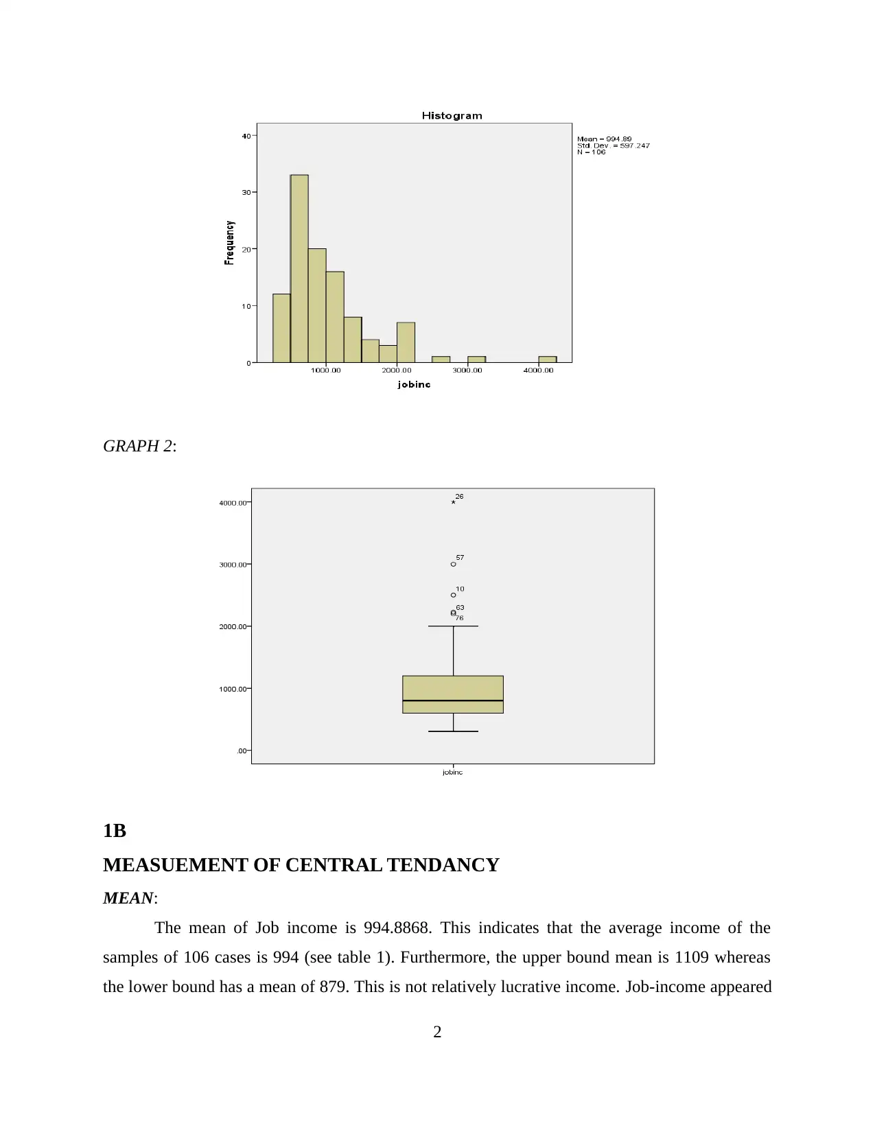
Graph 1, 2 and appendix 1 clearly indicates that the outcome of job income is positively
skewed. According to Field (2015), “there are two main ways in which a distribution can deviate
from normality”. The lack of symmetry which is known as skew is one and pointiness which is
known kurtosis is the second category. Both these categories are not normally distributed for job
income which further supports the positively skewed graphs (see graph 1 and 2). This suggests
that graphs are non-symmetrical therefore they are not normally distributed. Furthermore, table
one show that the skewness and kurtosis of 2.085 and 6.175 respectively are above the norm1
which is in-line with the graphs that indicated positively skewness and lack of normality. The
skewness of 2.085 indicates that the distribution is highly skewed (see graph one). Therefore,
some outliers need to be deleted to make at least moderate skewed. Furthermore, table 1
indicates that the majority of the group in the statistics is lower bound. Most groups that applied
the credit people who applied are on the low-income scale and just few are from higher-income
band the graphs indicate skewed distribution that indicates and suggest that the mean is farther
out in the long tail than is the median (Moore and McCabe 2003, p. 43)
GRAPH 1:
1Norm= The skewness and kurtosis norm are between -1 and 1 for skewness and between -4 and 4 for
kurtosis
1

GRAPH 2:
1B
MEASUEMENT OF CENTRAL TENDANCY
MEAN:
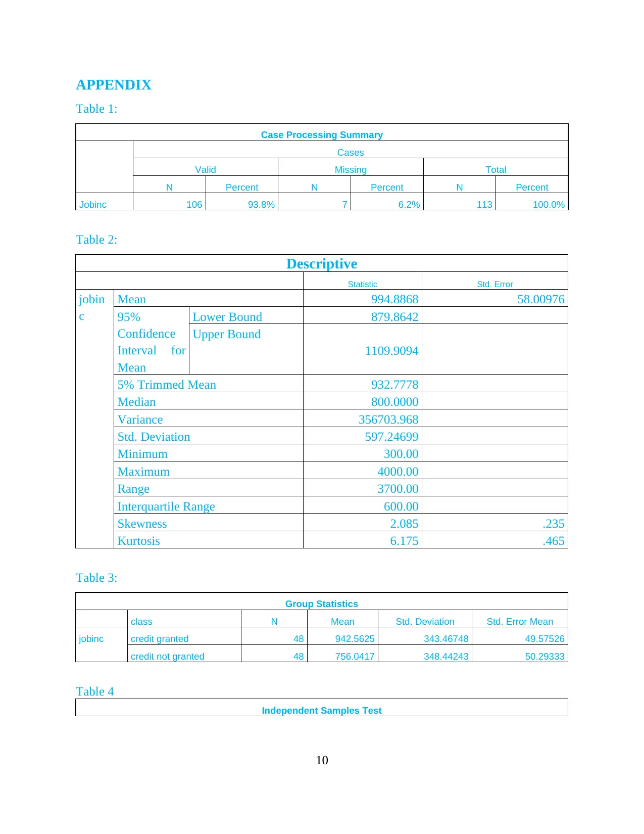
The mean of Job income is 994.8868. This indicates that the average income of the
samples of 106 cases is 994 (see table 1). Furthermore, the upper bound mean is 1109 whereas
the lower bound has a mean of 879. This is not relatively lucrative income. Job-income appeared
2

to be positively skewed distributed which implies that the mean lie towards the direction of skew
(the longer tail) relative to the median (Agresti and Finlay 1997, p. 50)
MEDIAN:
The median number that is separating the higher half of a job income data sample of
population from the lower half is 800. This further supports that it is not close to above
mentioned mean of close to 1000. That further supports the idea of non-normality distribution.
VARIANCE:
The measurement of distribution for job-income from the mean is 356703. This
Variance of measurement appears to be to be very high and one explanation could be high
number of outliers. This can be seen at Appendix 2. As the outliers, the variance came down
which indicates that it is in-line with the normal distribution. For instance, by the time the last
outlier of 46 is removed the variance goes down from 356,703 to 127, 220. That is staggering
64.33 % decrease. Still this indicates high variance from the mean.
STANDARD DEVIATION:
The standard deviation of Job income went from 597 before any outlier is deleted to 356
after all outliers is deleted. That is 40% decrease. Similarly, the variance correlates with outliers
and as the outliers are eliminated the standard deviation decreases. This is again in-line with
normality distribution as appendix 2 indicates.
Basic statistics are given below. It shows that there is considerable variation and
difference between the mean and medium value with high variance. The result also demonstrates
significant deviation from normality by giving the significant high level of positively skew. This
can be seen the skew result of 2.085.
As the descriptive (table 2) indicates that the Skewness is 2.085 which are above the
norm of between 1 and -1 as mentioned before. That further justifies the underlying principles of
removing outliers such as 26. Similarly, the Kurtosis is more than the norm of 4 which further
illustrates and supports the reason for deleting some outliers to make the distribution normal or
close to normality.
Using outlier labelling rule model if the g = 1.5 there are some outliers Tukey (1977).
With that in mind, the skewness and kurtosis are above the norm (-1 to 1 and -4 and 4) after the
first result it is suggested that some outliers should be removed to get to normality. The outliers
are 26, 56 and 10. Therefore, outliers are deleted one by one. The result indicates that the
3

skewness and kurtosis are going down but after deleting the first three that is 26, 56 and 10 the
kurtosis appear to be within the range but skewness is still slightly outside the range. Therefore,
further two outliers 60 and 72 are removed (see graph 2).
However, after removing 60, the result was reducing and it appears that there were only
one more outlier (72) (see appendix). Furthermore, after deleting 72 it created another 5 outliers
therefore further reduction occurred until the skewness goes below one. So the further outliers
such as (21, 4, 33, 38 and 46) were deleted before both the skewness and the kurtosis became
normal. However, the kurtosis was already within the norm by the time the third outlier 10 was
deleted. Furthermore, after 46 was deleted the Skewness and Kurtosis become 956 and 567
respectively which is well within the norm. After 46, no need to delete anymore outliers.
1C
A sample of 106 applicants is chosen to make inference about the population. These
inferences are based on mutually exclusive statement (Hypothesis). In order to determine this
inference a test is used to give basis for groups that are granted credit and those who are not
granted (see table 3). A sample of 96 was taken from the groups whether there is a significant
difference between the two groups
The result indicates that those who got credit appeared to have higher income than
unsuccessful once. Therefore, hypothesis testing is done to support or deny this claim.
 Ho: there is no significant difference in job-income mean between those who get credit
and those who did not
 Hi: Those who got credit got higher income.
It is worth knowing that if for-instance the Hi stands for there is a significant different
there is two tail (higher income or lower income). However, for simplicity the job-income T-test
will examine one tail test which is higher income. However, monthly incomes of those who get
credit and one who are unsuccessful are different. The successful once got higher income (see
table 3). This can be seen that the higher mean income of who granted credit compares to
unsuccessful one. The mean for successful and unsuccessful is 942 and 756 respectively.
As per table 3 and 4 in Appendix proved and based on the given rationale/parameters
there is a significant difference. Mean difference can be seen in the table 3. Therefore, we retain
the null hypothesis. This is because the alternative actual mean is currently 756 which are below
4

the null hypothesis (942). It can be said that, there is significant evidence that those who granted
the credit appeared to have higher income then than the other group.
Α= 5%
The significant associated with test of equality of variance is 0.013 and consequently, the
null hypothesis is accepted. In contrast, equally variance assumed line which gives 0 significant
is rejected. We reject the alternative since it is lower than 5% alpha. Because it is independent
now the test of variances is needed. The above table indicates that those who got credit and
those who did not get credit have higher difference in income. Since, now twe can change the
means of groups and the alternative. We reject not assume because it is lower than 5% which is
our level of acceptance. Furthermore, they are not homogeneous.
ASSUMPTIONS
 Normality of errors
 Homoscedasticity
 Independence of errors
 Linearity
According to Field (2015), the first head of the beast of bias is outliers. There appear to
be division of opinion regarding assumption of normality. Some believe that it is the mean that
your data need to be normally distributed. However, Field (2015) disagree that and believes that
assumption of normality might mean different things in different contexts. For example, the
confident intervals around a parameter estimate such as mean to be accurate, that estimate must
come from a normal distribution. Another angle is the significance test of models and the
parameter estimates which define them to be accurate the sampling distribution of what’s being
tested must be normal. However, the central limit theorem means that there are a variety of
situations in which we can assume normality regardless of the shape of our sample data (Lumley,
Diehr, Emersen, & Chen, 2002). However, If the attention is only to estimate the parameters of
the model in the sample like job-income, then homogeneity of variance in most cases is not
important or at-least not relevant. The method of least squares will produce unbiased estimates
(Hayes and Cai, 2007).
ONE WAY ANOVA
H1: There is no significant difference between any two means
5

Ho; At least there is a significant difference of two means
Within groups should be same as the table below proves otherwise they are not the same
group. Between groups should be large because they are from different group (see ANOVA table
10).
The significant is 0 and that means we reject the NUL hypothesis. This is simply the fact
that we have more than two mean test post hoc test is needed to identify these differences.
However, before post hoc is carried out so we need to test homogeneity of variance. Because we
have more than to means and their significant is 0, we reject the Null hypothesis above.
However, If Anova is simply a linear model than all of the potential sources of bias
shown below will be applied (Field, 2015).Therefore in order to reduce parsimony numbers
should not affect each other otherwise it will not be linear
 Additivity and Linearity
 Normality of something or others
 Homoscedasticity or homogeneity of variance
 Independence
TEST OF HOMOGENEITY OF VARIANCES
The output from the scheffe, Tukey and Gabriel shows that there are three different
groups. Group one comprises others and group second comprises of supervisory and group three
comprises of management. The result indicates that management got the highest income and
supervisory is second whereas others are the lowest. Therefore, our assumption that management
got higher income is confirmed. This result indicates that there significance is more than 10%,
therefore the report retained the result. It appears that management and supervisors show higher
income based on Gabriel, Scheffe and Tukey. They appeared to be good group since you cannot
break the group. However, regular check in needed in the future since their sample is different.
PART 2 REGRESSION
According to Filed and Hole (2003), “more often than not the manipulation of the
independent variable involves having an experimental condition and control group”. With that
in-mind, regression was used in this report to determine the statistical significance of class, sex,
age, job years, education Marital status, management and supervisors. Further, test was done to
determine the strength of association between job income and dependent variables and above
6

mentioned 8 independent variables. In addition, regression identified the relative importance of
each of the independent variables in predicting the single metric dependent variable of job-
income. For instance, as table 11 indicates job years, m-status and class are not relatively
important as compared to rest of the variables. That supports the reason they were eliminated in
later parts regression test, hence created reduced model. That proved that, the regression test
enabled to develop best model to explain job-income.
In addition to the above, this section will carry out multiple linear regressions with eight
independent variables assuming level of significance is 5%. The result of table 12 indicates that
R square value of around 81/5 which is reasonable. In addition to that, adjusted R square is very
close to R square especially when the non-influential variables such as class, marital status and
job years are removed. That said no concern regarding over fitting.
First model that fits:
Y ( jobinc)=bo +b 1 ( class ) +b 2 ( sex ) +b 3 ( age ) +b 4 ( job years ) + b 5 ( edu ) +b 6 ( mar status ) + b 7 ( managment ) + b 8 ( Su
The above two tables indicate that by deleting three non-influential independent variables
the model fit shown below is better that the original one that has been created.
From the output of ANOVA (Table 13 in Appendix) it can be seen that we reject the null
hypothesis and conclude that the R square is greater than zero or not all regression coefficient are
zero.
As the coefficient table below indicates that there are 5 independent variables that are
higher than 5% hence they are not significant to the job income. Since these are higher than 5%
deleting them will not affect the dependable variables of job-income as there is no correlation
between Y variables (job-income) and multiple independent variables (i.e job years, marital
status, class, age and sex), Therefore, the report deleted one by one depending on the higher
away they are from the 4%. For example, Job years is 0.747, marital status is 0.338, whereas
class is 0.274 and age is 0.230. Finally, sex is 0.021. This indicates that above are not relevant to
the job income. Similarly, it states that job status and education are the most relevant to the job
income or how much one can earn per month.
As (table 7 in Appendix) indicates that Class, age, job years and marital status are not
relevant to the job income since their significant is above the 5% norm. Therefore, job years is
eliminated first since it is the highest (74%). Then the marital status was removed second as it
7

now the highest of the remaining variables (34%). Finally, class which is (24) is also eliminated
since it is also higher than 5%. In-line with significant result, the standardized coefficients beta
of the removed variables are all less than the once that obtained. That is another reason for their
eliminations.
Y ( job income ) =bo+b 1 ( sex ) +b 2 ( age ) +b 3 ( educ ) +b 4 ( man ) + b5 (¿)
Effect size appeared to assist to determine which meaningful is more significant so job status has
large effect on income even though the management and supervisors significant is zero.
Based on coefficients (table 14) below there are 4 cases where there is significant. They
said items such as Sex, Education, Management and supervisors or job- status can influence your
job income. However, after removing only job years the age falls within the range. It falls from
23% to just 5% after removing job years. Furthermore, this improves the relationship between
age and job years. If any of the assumptions are not true usually referred to as a violation, then
the test static and p Values will be inaccurate and could lead us to the wrong conclusion if we
interpret them at the face value.
8

REFERENCE
Beyer, H. "Tukey, John W.: Exploratory Data Analysis. Addison-Wesley Publishing Company
Reading, Mass. — Menlo Park, Cal., London, Amsterdam, Don Mills, Ontario, Sydney
1977, XVI, 688 S.". Biom. J. 23.4 (1981): 413-414. Web. 22 Feb. 2016.
Decoster, Galluci, & Iselin, 2011; Decoster, Iselin, &Gallucci, 2009; MacCallum, et al., 2002.
Hippel, P, T, V., (2005) Amstat.org,. "Journal of Statistics Education, V13n2: Paul T. Von
Hippel". N.p., 2016. Web. 28 Feb. 2016.
Matthews, Patrick. "Median, Mode, Skewness, And Kurtosis In MS Access". Experts-
exchange.com. N.p., 2016. Web. 28 Feb. 2016.
9

APPENDIX
Table 1:
Case Processing Summary
Cases
Valid Missing Total
N Percent N Percent N Percent
Jobinc 106 93.8% 7 6.2% 113 100.0%
Table 2:
Descriptive
Statistic Std. Error
jobin
c
Mean 994.8868 58.00976
95%
Confidence
Interval for
Mean
Lower Bound 879.8642
Upper Bound
1109.9094
5% Trimmed Mean 932.7778
Median 800.0000
Variance 356703.968
Std. Deviation 597.24699
Minimum 300.00
Maximum 4000.00
Range 3700.00
Interquartile Range 600.00
Skewness 2.085 .235
Kurtosis 6.175 .465
Table 3:
Group Statistics
class N Mean Std. Deviation Std. Error Mean
jobinc credit granted 48 942.5625 343.46748 49.57526
credit not granted 48 756.0417 348.44243 50.29333
Table 4
Independent Samples Test
10