Statistical Analysis of Business Startup Costs and Sales Prediction

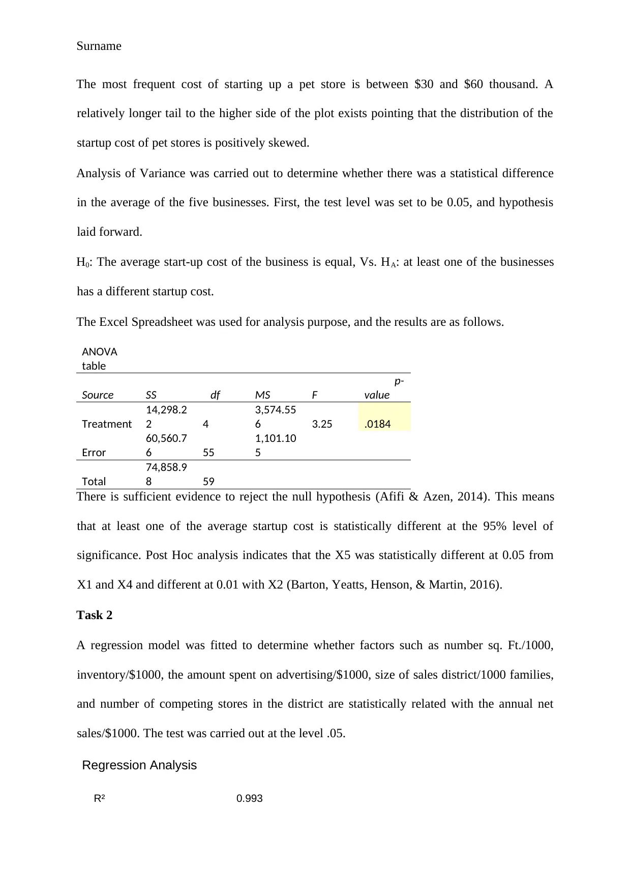
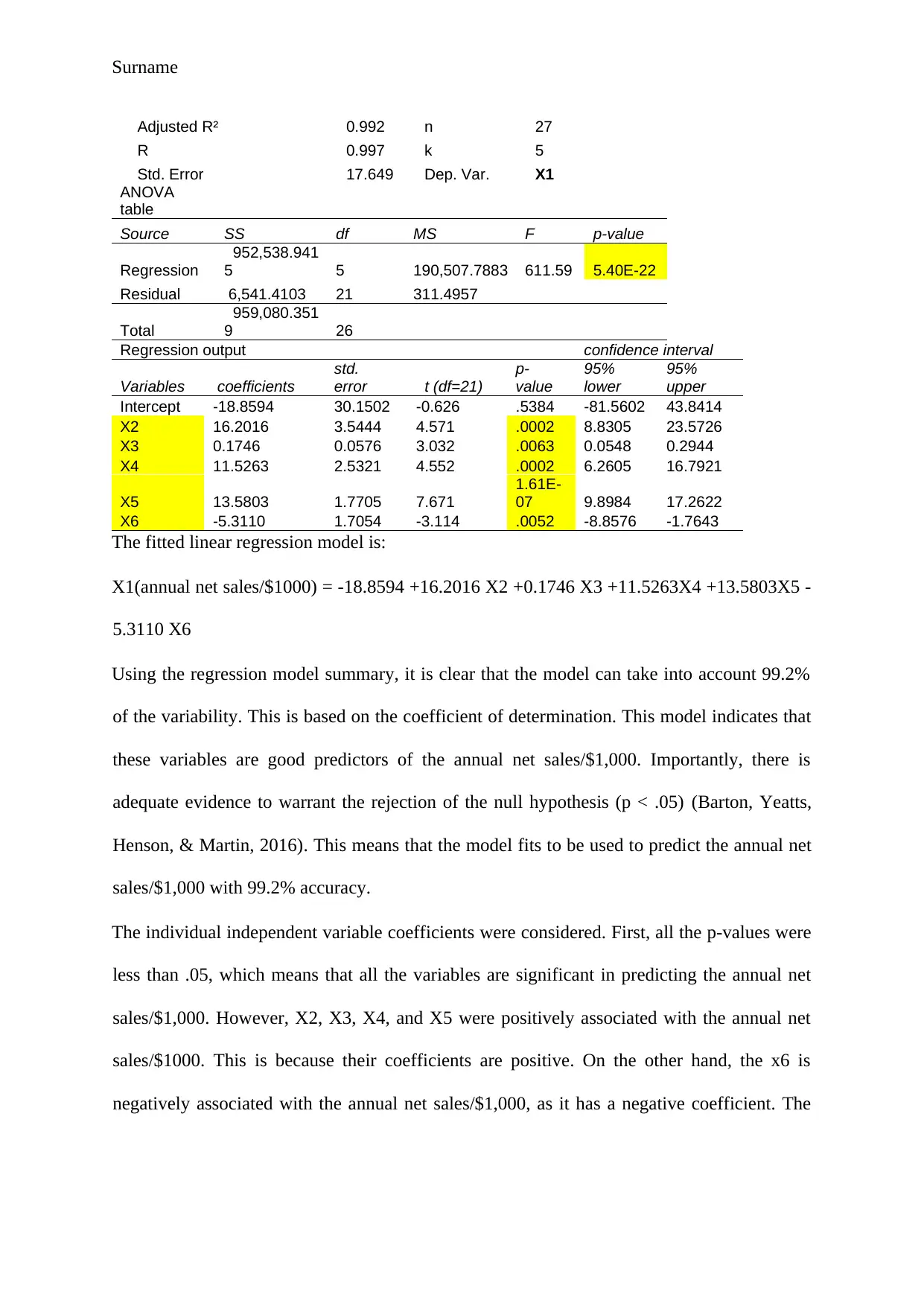
This project delves into a statistical analysis of business startup costs across five different types of shops: pizza, baker/donuts, shoe stores, gift shops, and pet stores. The analysis begins with descriptive statistics, including mean, median, mode, range, variance, standard deviation, and skewness, to understand the central tendencies and distributions of startup costs for each business type. Frequency distributions and histograms are used to visualize the data and identify patterns. An ANOVA test is conducted to determine if there are statistically significant differences in the average startup costs among the five businesses. Furthermore, a regression model is developed to assess the relationship between various factors, such as square footage, inventory, advertising spend, sales district size, and the number of competing stores, with annual net sales. The model's goodness-of-fit, significance of individual variables, and the ability to predict sales are evaluated. The project concludes with a practical application of the regression model to predict annual net sales based on specific input values. The findings highlight the statistical insights gained from the analysis and the predictive power of the regression model.

Surname
Statistics
Name
The Name of the Class (Course)
Professor (Tutor)
Name of the University
The City and State where it is located
Date

Surname
Task 1
The assessment in this part will evaluate basic descriptive statistics and the distribution of
business startup costs (thousands of dollars) for shops. This will help in understanding some
statistics of the business such as; startup costs for pizza, startup costs for baker/donuts,
startup costs for shoe stores, startup costs for gift shops, and startup costs for pet stores.
First, descriptive statistics were computed, and they are as summarized below.
X1 X2 X3 X4 X5
Mean 83 92.09 72.30 87.00 51.63
Median 80 87 70 97.5 49
Mode 35 #N/A #N/A 100 30
Minimum 35 40 35 35 20
Maximum 140 160 125 150 110
Range 105 120 90 115 90
Variance 1,165.17 1,512.69 983.79 1,289.11 733.05
Standard Deviation 34.13 38.89 31.37 35.90 27.07
Coeff. of Variation 41.13% 42.23% 43.38% 41.27% 52.45%
Skewness 0.1330 0.5098 0.5461 0.0773 0.6331
Kurtosis -1.0419 -0.4369 -0.9590 -0.4857 -0.4767
Count 13 11 10 10 16
Standard Error 9.4672 11.7268 9.9186 11.3539 6.7687
The average cost of starting up a pizza shop is $83 thousand, with a standard deviation of
34.13. The median of the startup cost of the pizza is slightly lower than the mean. The
difference between the highest cost and the least cost of starting up is $105. The average
startup costs for baker/donuts is $92.09 thousand with a standard deviation of $38.89
thousand. This average startup cost is slightly higher than the median, which is $87.00
thousand. This average is the highest among the five businesses start-up cost. An average of
$72.30 thousand is expected to be used as the startup costs for shoe stores, with a deviation of
$31.37 thousand from the mean. The startup costs for gift shops on average is $87.00
thousand with a standard deviation of $35.90 thousand. Lastly, the expected startup costs for
pet stores is $51.63 thousand, which is the least startup cost. This is the least startup cost, and
the standard deviation shows that the start-up cost for the pet store is more consistent.
The frequency tables with their respective histograms are as illustrated below.

Surname
Frequency Distribution - Quantitative
X1 cumulative
low
er
uppe
r midpoint width
frequenc
y percent
frequenc
y
percen
t
30 < 60 45 30 4 30.8 4 30.8
60 < 90 75 30 4 30.8 8 61.5
90 < 120 105 30 2 15.4 10 76.9
120 < 150 135 30 3 23.1 13 100.0
30
60
90
120
150
0
5
10
15
20
25
30
35
Histogram
X1
Percent
The chart indicates that most of the observations are on the lower side, with fewer businesses
costing between $90 and $120 thousands. The data seem to be skewed to the light, implying
that most of the observations on the lower side (left of the plot).
Frequency Distribution - Quantitative
X
2 cumulative
lower upper midpoint width frequency percent frequency percent
30 < 60 45 30 2 18.2 2 18.2
60 < 90 75 30 4 36.4 6 54.5
90 < 120 105 30 2 18.2 8 72.7
120 < 150 135 30 1 9.1 9 81.8
150 < 180 165 30 2 18.2 11 100.0
11 100.0

Surname
30
60
90
120
150
180
0
10
20
30
40
Histogram
X2
Percent
The histogram indicates that the most frequent business startup cost of baker/donuts lies
between $60 and $90 thousand. There appear to be fewer observations on the upper side of
the plot, deducing a positively skewed sample data.
Frequency Distribution - Quantitative
X
3 cumulative
lower upper midpoint width frequency percent frequency percent
30 < 60 45 30 4 40.0 4 40.0
60 < 90 75 30 3 30.0 7 70.0
90 < 120 105 30 2 20.0 9 90.0
120 < 150 135 30 1 10.0 10 100.0
10 100.0
30
60
90
120
150
0
10
20
30
40
50
Histogram
X3
Percent
The chart shows that most of the startup costs for shoe stores lie between $30 and $60
thousand. There is a progressive decline in the number of businesses opened with more
startup cost. This shows that the plot is positively skewed.
Frequency Distribution - Quantitative

Surname
X
4 cumulative
lower upper midpoint width frequency percent frequency percent
30 < 60 45 30 3 30.0 3 30.0
60 < 90 75 30 1 10.0 4 40.0
90 < 120 105 30 4 40.0 8 80.0
120 < 150 135 30 1 10.0 9 90.0
150 < 180 165 30 1 10.0 10 100.0
10 100.0
30
60
90
120
150
180
0
10
20
30
40
50
Histogram
X4
Percent
Most of the gift shops are started with cash between $90 and $120 thousand, followed by
those between $30 and $60 thousand. Since there are fewer observations on the upper side of
the plot, it is evident the plot is positively skewed.
Frequency Distribution - Quantitative
X
5 cumulative
lower upper midpoint width frequency percent frequency percent
0 < 30 15 30 4 25.0 4 25.0
30 < 60 45 30 6 37.5 10 62.5
60 < 90 75 30 5 31.3 15 93.8
90 < 120 105 30 1 6.3 16 100.0
16 100.0
0
30
60
90
120
0
10
20
30
40
Histogram
X5
Percent

Surname
The most frequent cost of starting up a pet store is between $30 and $60 thousand. A
relatively longer tail to the higher side of the plot exists pointing that the distribution of the
startup cost of pet stores is positively skewed.
Analysis of Variance was carried out to determine whether there was a statistical difference
in the average of the five businesses. First, the test level was set to be 0.05, and hypothesis
laid forward.
H0: The average start-up cost of the business is equal, Vs. HA: at least one of the businesses
has a different startup cost.
The Excel Spreadsheet was used for analysis purpose, and the results are as follows.
ANOVA
table
Source SS df MS F
p-
value
Treatment
14,298.2
2 4
3,574.55
6 3.25 .0184
Error
60,560.7
6 55
1,101.10
5
Total
74,858.9
8 59
There is sufficient evidence to reject the null hypothesis (Afifi & Azen, 2014). This means
that at least one of the average startup cost is statistically different at the 95% level of
significance. Post Hoc analysis indicates that the X5 was statistically different at 0.05 from
X1 and X4 and different at 0.01 with X2 (Barton, Yeatts, Henson, & Martin, 2016).
Task 2
A regression model was fitted to determine whether factors such as number sq. Ft./1000,
inventory/$1000, the amount spent on advertising/$1000, size of sales district/1000 families,
and number of competing stores in the district are statistically related with the annual net
sales/$1000. The test was carried out at the level .05.
Regression Analysis
R² 0.993

Surname
Adjusted R² 0.992 n 27
R 0.997 k 5
Std. Error 17.649 Dep. Var. X1
ANOVA
table
Source SS df MS F p-value
Regression
952,538.941
5 5 190,507.7883 611.59 5.40E-22
Residual 6,541.4103 21 311.4957
Total
959,080.351
9 26
Regression output confidence interval
Variables coefficients
std.
error t (df=21)
p-
value
95%
lower
95%
upper
Intercept -18.8594 30.1502 -0.626 .5384 -81.5602 43.8414
X2 16.2016 3.5444 4.571 .0002 8.8305 23.5726
X3 0.1746 0.0576 3.032 .0063 0.0548 0.2944
X4 11.5263 2.5321 4.552 .0002 6.2605 16.7921
X5 13.5803 1.7705 7.671
1.61E-
07 9.8984 17.2622
X6 -5.3110 1.7054 -3.114 .0052 -8.8576 -1.7643
The fitted linear regression model is:
X1(annual net sales/$1000) = -18.8594 +16.2016 X2 +0.1746 X3 +11.5263X4 +13.5803X5 -
5.3110 X6
Using the regression model summary, it is clear that the model can take into account 99.2%
of the variability. This is based on the coefficient of determination. This model indicates that
these variables are good predictors of the annual net sales/$1,000. Importantly, there is
adequate evidence to warrant the rejection of the null hypothesis (p < .05) (Barton, Yeatts,
Henson, & Martin, 2016). This means that the model fits to be used to predict the annual net
sales/$1,000 with 99.2% accuracy.
The individual independent variable coefficients were considered. First, all the p-values were
less than .05, which means that all the variables are significant in predicting the annual net
sales/$1,000. However, X2, X3, X4, and X5 were positively associated with the annual net
sales/$1000. This is because their coefficients are positive. On the other hand, the x6 is
negatively associated with the annual net sales/$1,000, as it has a negative coefficient. The

Surname
table also indicates that since the 95% confidence interval does not contain zero, it means that
the coefficients are significant. That is, they are significantly different from zero.
Since all the independent variables are significant, there is no need to remodel a linear
regression model. Thus, we use the given model to predict the net sales/$1,000 using the
regression model.
Net sales/$1000 = -18.8594 + 16.2016 X2+0.1746X3 + 11.5263 X4 +13.5803X5 - 5.3110
X6; when;
X2 = number sq. ft./1000 = $1000
X3 = inventory/$1000 = $150,000
X4 = amount spent on advertising/$1000 = $5000
X5 = size of sales district/1000 families = 5000
X6 = number of competing stores in district = 2
= -18.8594 + 16.2016 (1000) + 0.1746(150,000) + 11.5263(5000) +13.5803(1000) -
5.3110(2)
= 167,900.2749997
The sale will be approximately 167,900.27

Surname
References
Afifi, A. A., & Azen, S. P. (2014). Statistical analysis: a computer oriented approach.
Academic press.
Barton, M., Yeatts, P. E., Henson, R. K., & Martin, S. B. (2016). Moving beyond univariate
post-hoc testing in exercise science: A primer on descriptive discriminate analysis.
Research quarterly for exercise and sport, 87(4), 365-375.
Chatterjee, S., & Hadi., A. S. (2015). Regression analysis by example. John Wiley & Sons.