A Statistical Analysis of Factors Affecting Students' Performance
VerifiedAdded on 2022/11/14
|15
|3179
|108
Report
AI Summary
This report presents a statistical analysis of factors affecting student performance, based on a sample of 50 students. The research investigates the impact of major (Accounting vs. Business), gender, and study habits on academic outcomes. Descriptive statistics reveal the distribution of students across majors and genders, along with grade distributions. Inferential statistics, including confidence intervals and ANOVA, are used to compare study habits and working hours between different groups. Regression analysis is employed to examine the relationship between study hours and final scores, as well as the relationship between study hours and work hours. Key findings indicate that accounting majors generally performed better than business majors and that female students performed better than male students. The analysis also reveals a positive correlation between study hours and final scores, but no significant relationship between study hours and working hours. The report concludes with a discussion of the implications of these findings.
Running head: STUDENTS’ PERFORMANCE 1
Factors Affecting Students’ Performance
Name:
Institution:
Factors Affecting Students’ Performance
Name:
Institution:
Paraphrase This Document
Need a fresh take? Get an instant paraphrase of this document with our AI Paraphraser
STUDENTS’ PERFORMANCE 2
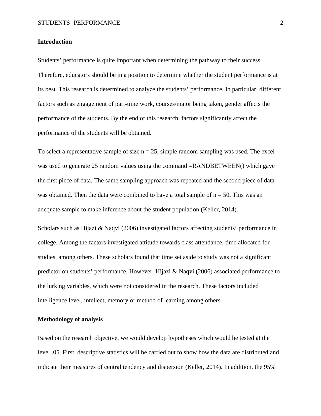
Introduction
Students’ performance is quite important when determining the pathway to their success.
Therefore, educators should be in a position to determine whether the student performance is at
its best. This research is determined to analyze the students’ performance. In particular, different
factors such as engagement of part-time work, courses/major being taken, gender affects the
performance of the students. By the end of this research, factors significantly affect the
performance of the students will be obtained.
To select a representative sample of size n = 25, simple random sampling was used. The excel
was used to generate 25 random values using the command =RANDBETWEEN() which gave
the first piece of data. The same sampling approach was repeated and the second piece of data
was obtained. Then the data were combined to have a total sample of n = 50. This was an
adequate sample to make inference about the student population (Keller, 2014).
Scholars such as Hijazi & Naqvi (2006) investigated factors affecting students’ performance in
college. Among the factors investigated attitude towards class attendance, time allocated for
studies, among others. These scholars found that time set aside to study was not a significant
predictor on students’ performance. However, Hijazi & Naqvi (2006) associated performance to
the lurking variables, which were not considered in the research. These factors included
intelligence level, intellect, memory or method of learning among others.
Methodology of analysis
Based on the research objective, we would develop hypotheses which would be tested at the
level .05. First, descriptive statistics will be carried out to show how the data are distributed and
indicate their measures of central tendency and dispersion (Keller, 2014). In addition, the 95%
STUDENTS’ PERFORMANCE 3
confidence interval will be constructed to show the range at which the population parameters are
expected to lie between. Also, hypothesis for the difference of the means between groups will be
tested. Most importantly, effects of different factors on students’ performance will be
investigated. The results section will be subdivided into two sections, where the first one will
contain descriptive statistics and the second inferential statistics.
Results
Descriptive statistics
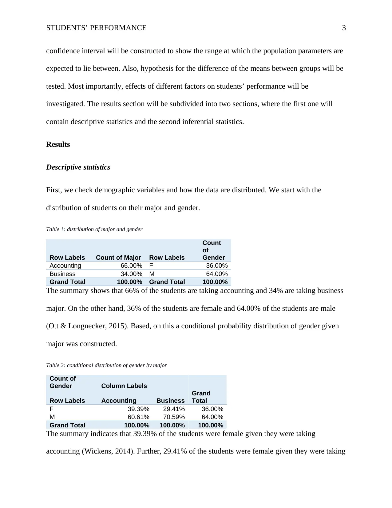
First, we check demographic variables and how the data are distributed. We start with the
distribution of students on their major and gender.
Table 1: distribution of major and gender
Row Labels Count of Major Row Labels
Count
of
Gender
Accounting 66.00% F 36.00%
Business 34.00% M 64.00%
Grand Total 100.00% Grand Total 100.00%
The summary shows that 66% of the students are taking accounting and 34% are taking business
major. On the other hand, 36% of the students are female and 64.00% of the students are male
(Ott & Longnecker, 2015). Based, on this a conditional probability distribution of gender given
major was constructed.
Table 2: conditional distribution of gender by major
Count of
Gender Column Labels
Row Labels Accounting Business
Grand
Total
F 39.39% 29.41% 36.00%
M 60.61% 70.59% 64.00%
Grand Total 100.00% 100.00% 100.00%
The summary indicates that 39.39% of the students were female given they were taking
accounting (Wickens, 2014). Further, 29.41% of the students were female given they were taking
confidence interval will be constructed to show the range at which the population parameters are
expected to lie between. Also, hypothesis for the difference of the means between groups will be
tested. Most importantly, effects of different factors on students’ performance will be
investigated. The results section will be subdivided into two sections, where the first one will
contain descriptive statistics and the second inferential statistics.
Results
Descriptive statistics
First, we check demographic variables and how the data are distributed. We start with the
distribution of students on their major and gender.
Table 1: distribution of major and gender
Row Labels Count of Major Row Labels
Count
of
Gender
Accounting 66.00% F 36.00%
Business 34.00% M 64.00%
Grand Total 100.00% Grand Total 100.00%
The summary shows that 66% of the students are taking accounting and 34% are taking business
major. On the other hand, 36% of the students are female and 64.00% of the students are male
(Ott & Longnecker, 2015). Based, on this a conditional probability distribution of gender given
major was constructed.
Table 2: conditional distribution of gender by major
Count of
Gender Column Labels
Row Labels Accounting Business
Grand
Total
F 39.39% 29.41% 36.00%
M 60.61% 70.59% 64.00%
Grand Total 100.00% 100.00% 100.00%
The summary indicates that 39.39% of the students were female given they were taking
accounting (Wickens, 2014). Further, 29.41% of the students were female given they were taking
⊘ This is a preview!⊘
Do you want full access?
Subscribe today to unlock all pages.
Trusted by 1+ million students worldwide
STUDENTS’ PERFORMANCE 4
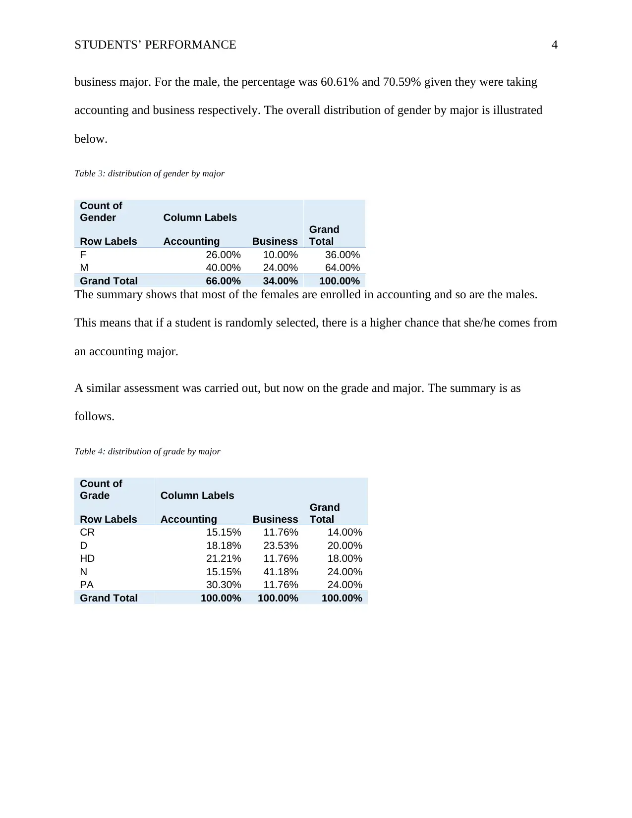
business major. For the male, the percentage was 60.61% and 70.59% given they were taking
accounting and business respectively. The overall distribution of gender by major is illustrated
below.
Table 3: distribution of gender by major
Count of
Gender Column Labels
Row Labels Accounting Business
Grand
Total
F 26.00% 10.00% 36.00%
M 40.00% 24.00% 64.00%
Grand Total 66.00% 34.00% 100.00%
The summary shows that most of the females are enrolled in accounting and so are the males.
This means that if a student is randomly selected, there is a higher chance that she/he comes from
an accounting major.
A similar assessment was carried out, but now on the grade and major. The summary is as
follows.
Table 4: distribution of grade by major
Count of
Grade Column Labels
Row Labels Accounting Business
Grand
Total
CR 15.15% 11.76% 14.00%
D 18.18% 23.53% 20.00%
HD 21.21% 11.76% 18.00%
N 15.15% 41.18% 24.00%
PA 30.30% 11.76% 24.00%
Grand Total 100.00% 100.00% 100.00%
Paraphrase This Document
Need a fresh take? Get an instant paraphrase of this document with our AI Paraphraser
STUDENTS’ PERFORMANCE 5
CR D HD N PA
0.00%
10.00%
20.00%
30.00%
40.00%
50.00%
Percentage of students by grade and major
Accounting
Business
grade
Percentage
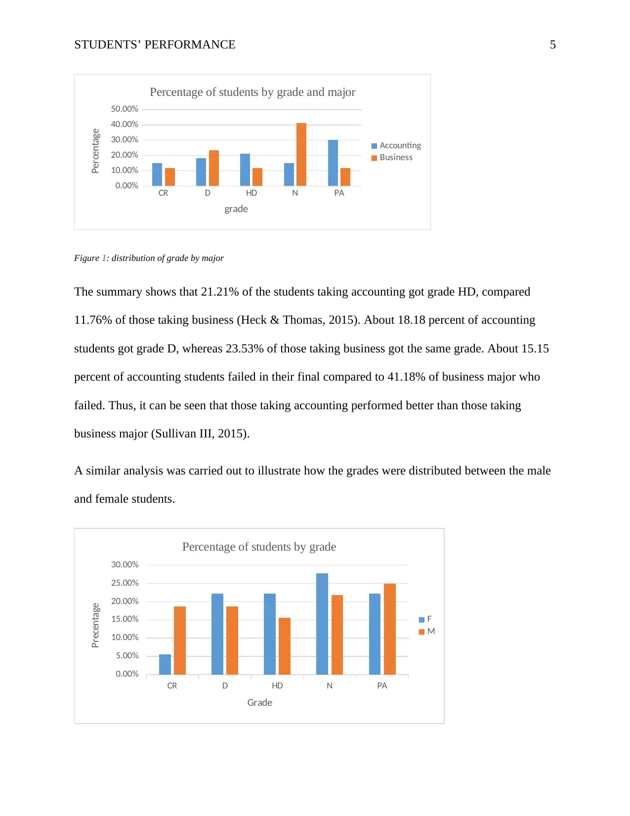
Figure 1: distribution of grade by major
The summary shows that 21.21% of the students taking accounting got grade HD, compared
11.76% of those taking business (Heck & Thomas, 2015). About 18.18 percent of accounting
students got grade D, whereas 23.53% of those taking business got the same grade. About 15.15
percent of accounting students failed in their final compared to 41.18% of business major who
failed. Thus, it can be seen that those taking accounting performed better than those taking
business major (Sullivan III, 2015).
A similar analysis was carried out to illustrate how the grades were distributed between the male
and female students.
CR D HD N PA
0.00%
5.00%
10.00%
15.00%
20.00%
25.00%
30.00%
Percentage of students by grade
F
M
Grade
Precentage
CR D HD N PA
0.00%
10.00%
20.00%
30.00%
40.00%
50.00%
Percentage of students by grade and major
Accounting
Business
grade
Percentage
Figure 1: distribution of grade by major
The summary shows that 21.21% of the students taking accounting got grade HD, compared
11.76% of those taking business (Heck & Thomas, 2015). About 18.18 percent of accounting
students got grade D, whereas 23.53% of those taking business got the same grade. About 15.15
percent of accounting students failed in their final compared to 41.18% of business major who
failed. Thus, it can be seen that those taking accounting performed better than those taking
business major (Sullivan III, 2015).
A similar analysis was carried out to illustrate how the grades were distributed between the male
and female students.
CR D HD N PA
0.00%
5.00%
10.00%
15.00%
20.00%
25.00%
30.00%
Percentage of students by grade
F
M
Grade
Precentage
STUDENTS’ PERFORMANCE 6
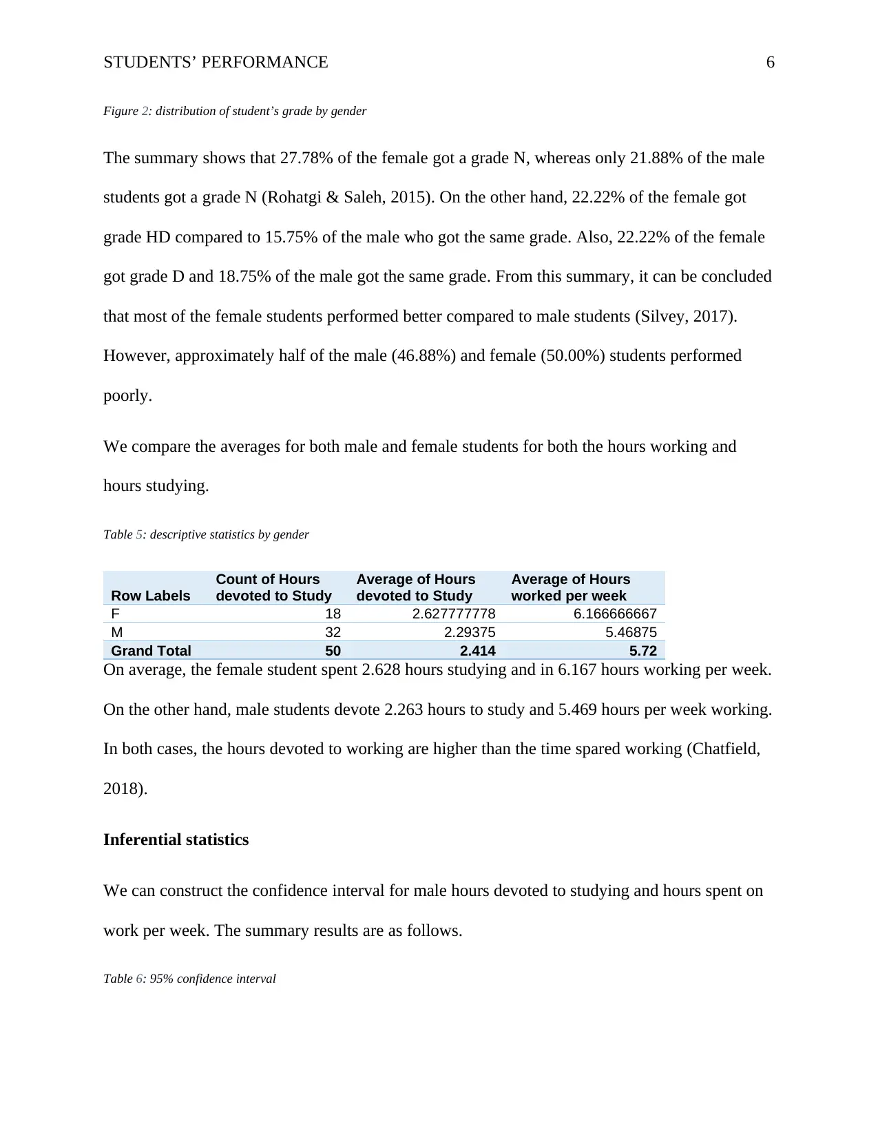
Figure 2: distribution of student’s grade by gender
The summary shows that 27.78% of the female got a grade N, whereas only 21.88% of the male
students got a grade N (Rohatgi & Saleh, 2015). On the other hand, 22.22% of the female got
grade HD compared to 15.75% of the male who got the same grade. Also, 22.22% of the female
got grade D and 18.75% of the male got the same grade. From this summary, it can be concluded
that most of the female students performed better compared to male students (Silvey, 2017).
However, approximately half of the male (46.88%) and female (50.00%) students performed
poorly.
We compare the averages for both male and female students for both the hours working and
hours studying.
Table 5: descriptive statistics by gender
Row Labels
Count of Hours
devoted to Study
Average of Hours
devoted to Study
Average of Hours
worked per week
F 18 2.627777778 6.166666667
M 32 2.29375 5.46875
Grand Total 50 2.414 5.72
On average, the female student spent 2.628 hours studying and in 6.167 hours working per week.
On the other hand, male students devote 2.263 hours to study and 5.469 hours per week working.
In both cases, the hours devoted to working are higher than the time spared working (Chatfield,
2018).
Inferential statistics
We can construct the confidence interval for male hours devoted to studying and hours spent on
work per week. The summary results are as follows.
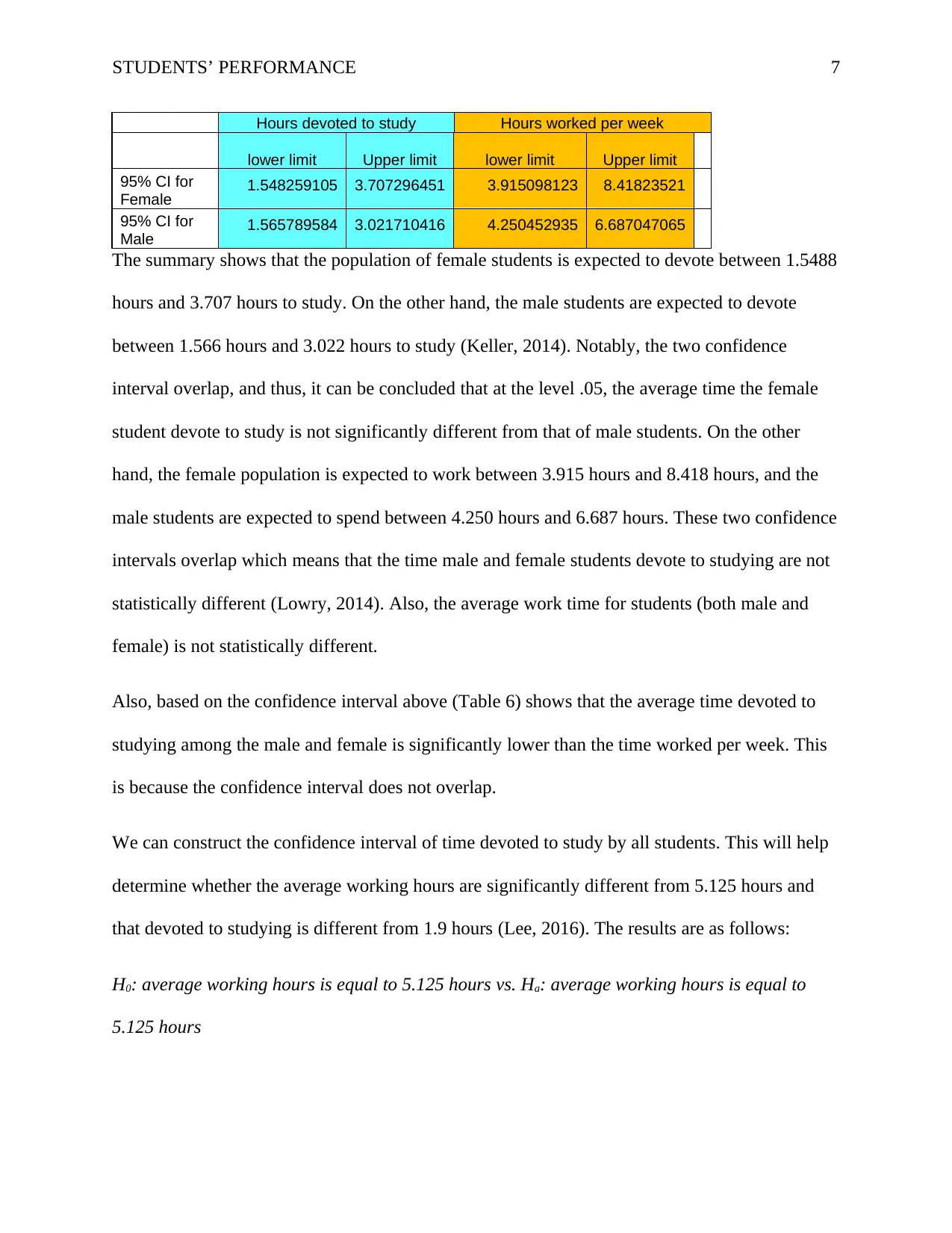
Table 6: 95% confidence interval
Figure 2: distribution of student’s grade by gender
The summary shows that 27.78% of the female got a grade N, whereas only 21.88% of the male
students got a grade N (Rohatgi & Saleh, 2015). On the other hand, 22.22% of the female got
grade HD compared to 15.75% of the male who got the same grade. Also, 22.22% of the female
got grade D and 18.75% of the male got the same grade. From this summary, it can be concluded
that most of the female students performed better compared to male students (Silvey, 2017).
However, approximately half of the male (46.88%) and female (50.00%) students performed
poorly.
We compare the averages for both male and female students for both the hours working and
hours studying.
Table 5: descriptive statistics by gender
Row Labels
Count of Hours
devoted to Study
Average of Hours
devoted to Study
Average of Hours
worked per week
F 18 2.627777778 6.166666667
M 32 2.29375 5.46875
Grand Total 50 2.414 5.72
On average, the female student spent 2.628 hours studying and in 6.167 hours working per week.
On the other hand, male students devote 2.263 hours to study and 5.469 hours per week working.
In both cases, the hours devoted to working are higher than the time spared working (Chatfield,
2018).
Inferential statistics
We can construct the confidence interval for male hours devoted to studying and hours spent on
work per week. The summary results are as follows.
Table 6: 95% confidence interval
⊘ This is a preview!⊘
Do you want full access?
Subscribe today to unlock all pages.
Trusted by 1+ million students worldwide
STUDENTS’ PERFORMANCE 7
Hours devoted to study Hours worked per week
lower limit Upper limit lower limit Upper limit
95% CI for
Female 1.548259105 3.707296451 3.915098123 8.41823521
95% CI for
Male 1.565789584 3.021710416 4.250452935 6.687047065
The summary shows that the population of female students is expected to devote between 1.5488
hours and 3.707 hours to study. On the other hand, the male students are expected to devote
between 1.566 hours and 3.022 hours to study (Keller, 2014). Notably, the two confidence
interval overlap, and thus, it can be concluded that at the level .05, the average time the female
student devote to study is not significantly different from that of male students. On the other
hand, the female population is expected to work between 3.915 hours and 8.418 hours, and the
male students are expected to spend between 4.250 hours and 6.687 hours. These two confidence
intervals overlap which means that the time male and female students devote to studying are not
statistically different (Lowry, 2014). Also, the average work time for students (both male and
female) is not statistically different.
Also, based on the confidence interval above (Table 6) shows that the average time devoted to
studying among the male and female is significantly lower than the time worked per week. This
is because the confidence interval does not overlap.
We can construct the confidence interval of time devoted to study by all students. This will help
determine whether the average working hours are significantly different from 5.125 hours and
that devoted to studying is different from 1.9 hours (Lee, 2016). The results are as follows:
H0: average working hours is equal to 5.125 hours vs. Ha: average working hours is equal to
5.125 hours
Paraphrase This Document
Need a fresh take? Get an instant paraphrase of this document with our AI Paraphraser
STUDENTS’ PERFORMANCE 8
H0: average devoted hours of study is equal to 1.9 hours vs. Ha: average devoted hours of study
is equal to 1.9 hours
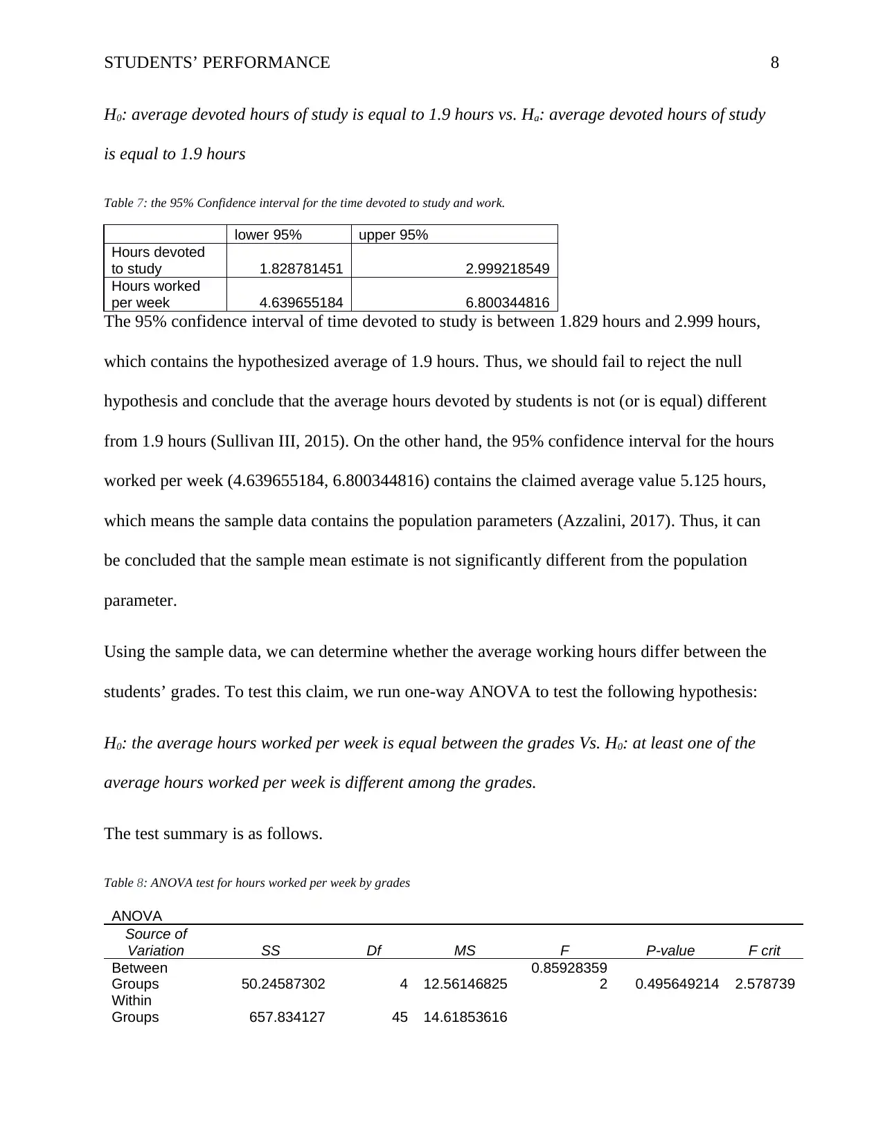
Table 7: the 95% Confidence interval for the time devoted to study and work.
lower 95% upper 95%
Hours devoted
to study 1.828781451 2.999218549
Hours worked
per week 4.639655184 6.800344816
The 95% confidence interval of time devoted to study is between 1.829 hours and 2.999 hours,
which contains the hypothesized average of 1.9 hours. Thus, we should fail to reject the null
hypothesis and conclude that the average hours devoted by students is not (or is equal) different
from 1.9 hours (Sullivan III, 2015). On the other hand, the 95% confidence interval for the hours
worked per week (4.639655184, 6.800344816) contains the claimed average value 5.125 hours,
which means the sample data contains the population parameters (Azzalini, 2017). Thus, it can
be concluded that the sample mean estimate is not significantly different from the population
parameter.
Using the sample data, we can determine whether the average working hours differ between the
students’ grades. To test this claim, we run one-way ANOVA to test the following hypothesis:
H0: the average hours worked per week is equal between the grades Vs. H0: at least one of the
average hours worked per week is different among the grades.
The test summary is as follows.
Table 8: ANOVA test for hours worked per week by grades
ANOVA
Source of
Variation SS Df MS F P-value F crit
Between
Groups 50.24587302 4 12.56146825
0.85928359
2 0.495649214 2.578739
Within
Groups 657.834127 45 14.61853616
H0: average devoted hours of study is equal to 1.9 hours vs. Ha: average devoted hours of study
is equal to 1.9 hours
Table 7: the 95% Confidence interval for the time devoted to study and work.
lower 95% upper 95%
Hours devoted
to study 1.828781451 2.999218549
Hours worked
per week 4.639655184 6.800344816
The 95% confidence interval of time devoted to study is between 1.829 hours and 2.999 hours,
which contains the hypothesized average of 1.9 hours. Thus, we should fail to reject the null
hypothesis and conclude that the average hours devoted by students is not (or is equal) different
from 1.9 hours (Sullivan III, 2015). On the other hand, the 95% confidence interval for the hours
worked per week (4.639655184, 6.800344816) contains the claimed average value 5.125 hours,
which means the sample data contains the population parameters (Azzalini, 2017). Thus, it can
be concluded that the sample mean estimate is not significantly different from the population
parameter.
Using the sample data, we can determine whether the average working hours differ between the
students’ grades. To test this claim, we run one-way ANOVA to test the following hypothesis:
H0: the average hours worked per week is equal between the grades Vs. H0: at least one of the
average hours worked per week is different among the grades.
The test summary is as follows.
Table 8: ANOVA test for hours worked per week by grades
ANOVA
Source of
Variation SS Df MS F P-value F crit
Between
Groups 50.24587302 4 12.56146825
0.85928359
2 0.495649214 2.578739
Within
Groups 657.834127 45 14.61853616
STUDENTS’ PERFORMANCE 9
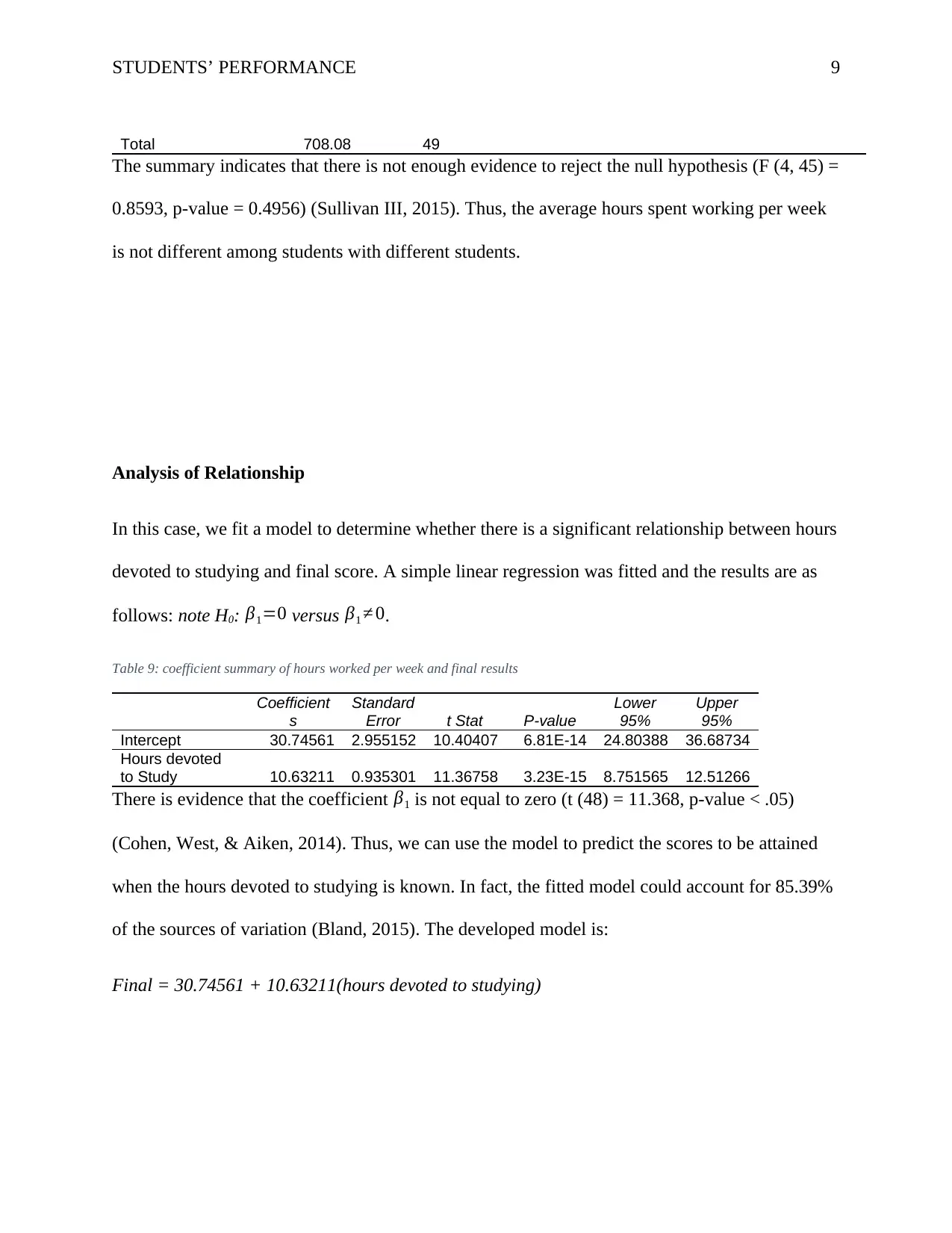
Total 708.08 49
The summary indicates that there is not enough evidence to reject the null hypothesis (F (4, 45) =
0.8593, p-value = 0.4956) (Sullivan III, 2015). Thus, the average hours spent working per week
is not different among students with different students.
Analysis of Relationship
In this case, we fit a model to determine whether there is a significant relationship between hours
devoted to studying and final score. A simple linear regression was fitted and the results are as
follows: note H0: β1=0 versus β1 ≠ 0.
Table 9: coefficient summary of hours worked per week and final results
Coefficient
s
Standard
Error t Stat P-value
Lower
95%
Upper
95%
Intercept 30.74561 2.955152 10.40407 6.81E-14 24.80388 36.68734
Hours devoted
to Study 10.63211 0.935301 11.36758 3.23E-15 8.751565 12.51266
There is evidence that the coefficient β1 is not equal to zero (t (48) = 11.368, p-value < .05)
(Cohen, West, & Aiken, 2014). Thus, we can use the model to predict the scores to be attained
when the hours devoted to studying is known. In fact, the fitted model could account for 85.39%
of the sources of variation (Bland, 2015). The developed model is:
Final = 30.74561 + 10.63211(hours devoted to studying)
⊘ This is a preview!⊘
Do you want full access?
Subscribe today to unlock all pages.
Trusted by 1+ million students worldwide
STUDENTS’ PERFORMANCE 10
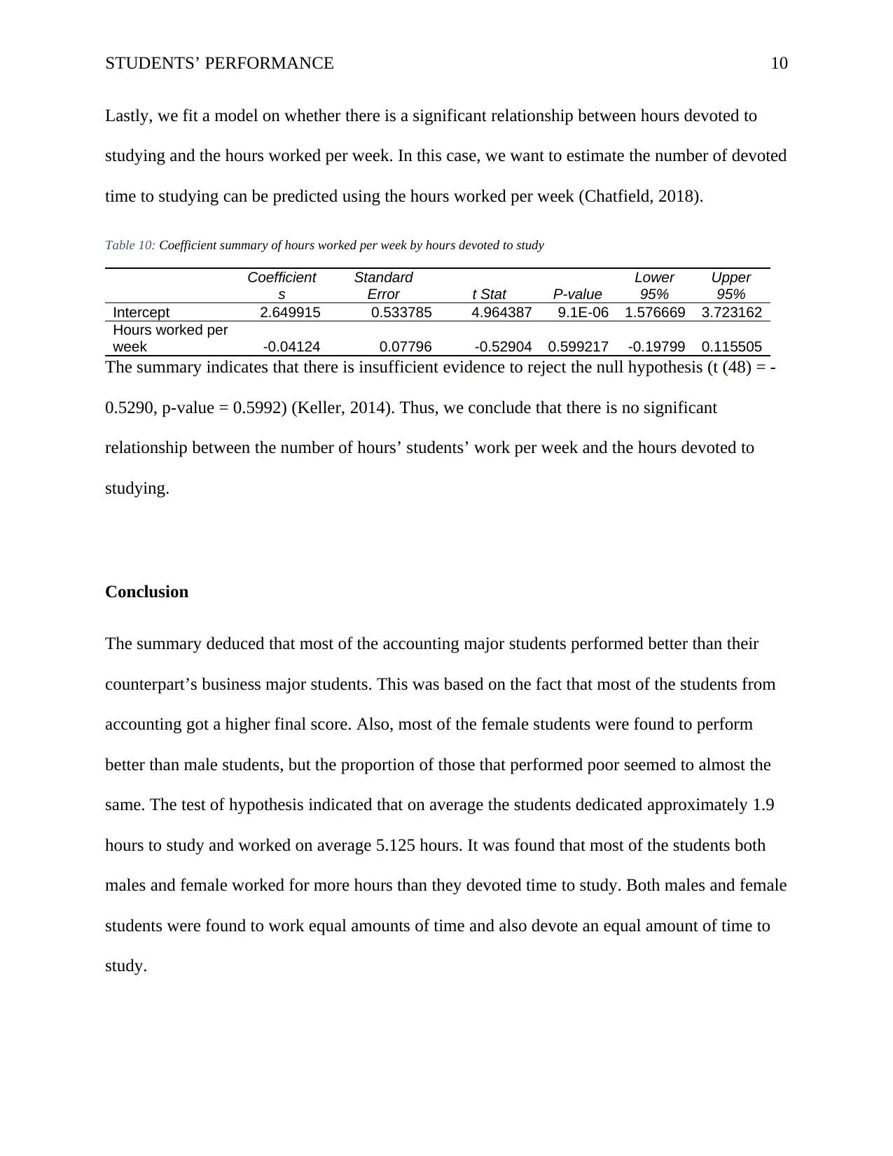
Lastly, we fit a model on whether there is a significant relationship between hours devoted to
studying and the hours worked per week. In this case, we want to estimate the number of devoted
time to studying can be predicted using the hours worked per week (Chatfield, 2018).
Table 10: Coefficient summary of hours worked per week by hours devoted to study
Coefficient
s
Standard
Error t Stat P-value
Lower
95%
Upper
95%
Intercept 2.649915 0.533785 4.964387 9.1E-06 1.576669 3.723162
Hours worked per
week -0.04124 0.07796 -0.52904 0.599217 -0.19799 0.115505
The summary indicates that there is insufficient evidence to reject the null hypothesis (t (48) = -
0.5290, p-value = 0.5992) (Keller, 2014). Thus, we conclude that there is no significant
relationship between the number of hours’ students’ work per week and the hours devoted to
studying.
Conclusion
The summary deduced that most of the accounting major students performed better than their
counterpart’s business major students. This was based on the fact that most of the students from
accounting got a higher final score. Also, most of the female students were found to perform
better than male students, but the proportion of those that performed poor seemed to almost the
same. The test of hypothesis indicated that on average the students dedicated approximately 1.9
hours to study and worked on average 5.125 hours. It was found that most of the students both
males and female worked for more hours than they devoted time to study. Both males and female
students were found to work equal amounts of time and also devote an equal amount of time to
study.
Paraphrase This Document
Need a fresh take? Get an instant paraphrase of this document with our AI Paraphraser
STUDENTS’ PERFORMANCE 11
When the relation assessment was carried out, it was found that the final score could be predicted
using the number of hours dedicated to study. However, it was found that the grades a student
score is not related to the hours dedicated to study. Nonetheless, it was established that there was
no relationship between hours spent working per week and the hours dedicated.
STUDENTS’ PERFORMANCE 12
References
Azzalini, A. (2017). Azzalini, A. (2017). Statistical inference based on the likelihood. Routledge.
Bland, M. (2015). n introduction to medical statistics. Oxford University Press (UK).
Chatfield, C. (2018). Statistics for technology: a course in applied statistics (3rd Edition ed.).
New York: Routledge.
Cohen, P., West, S. G., & Aiken, L. S. (2014). Applied multiple regression/correlation analysis
for the behavioral sciences (2nd ed.). Psychology Press.
Heck, R. H., & Thomas, S. L. (2015). An introduction to multilevel modeling techniques; MLM
and SEM approaches using Mplus. Routledge.
Hijazi, S. T., & Naqvi., S. M. (2006). FACTORS AFFECTING STUDENTS’
PERFORMANCE. Bangladesh e-Journal of Sociology, 3(1), 1 -10.
Keller, G. (2014). Statistics for Management and Economics (10th ed.). Stamford: Cengage
Learning.
Lee, D. K. (2016). Alternatives to P value: confidence interval and effect size. Korean journal of
anesthesiology, 69(6), 555.
Lowry, R. (2014). Concepts and applications of inferential statistics.
Ott, R. L., & Longnecker, M. T. (2015). An introduction to statistical methods and data analysis.
Nelson Education.
Rohatgi, V. K., & Saleh, A. M. (2015). An introduction to probability and statistics. John Wiley
& Sons.
⊘ This is a preview!⊘
Do you want full access?
Subscribe today to unlock all pages.
Trusted by 1+ million students worldwide
1 out of 15
Related Documents


Your All-in-One AI-Powered Toolkit for Academic Success.
+13062052269
info@desklib.com
Available 24*7 on WhatsApp / Email
![[object Object]](/_next/static/media/star-bottom.7253800d.svg)
Unlock your academic potential
Copyright © 2020–2026 A2Z Services. All Rights Reserved. Developed and managed by ZUCOL.