Data Analysis Assignment: Statistical Tests and Results Interpretation

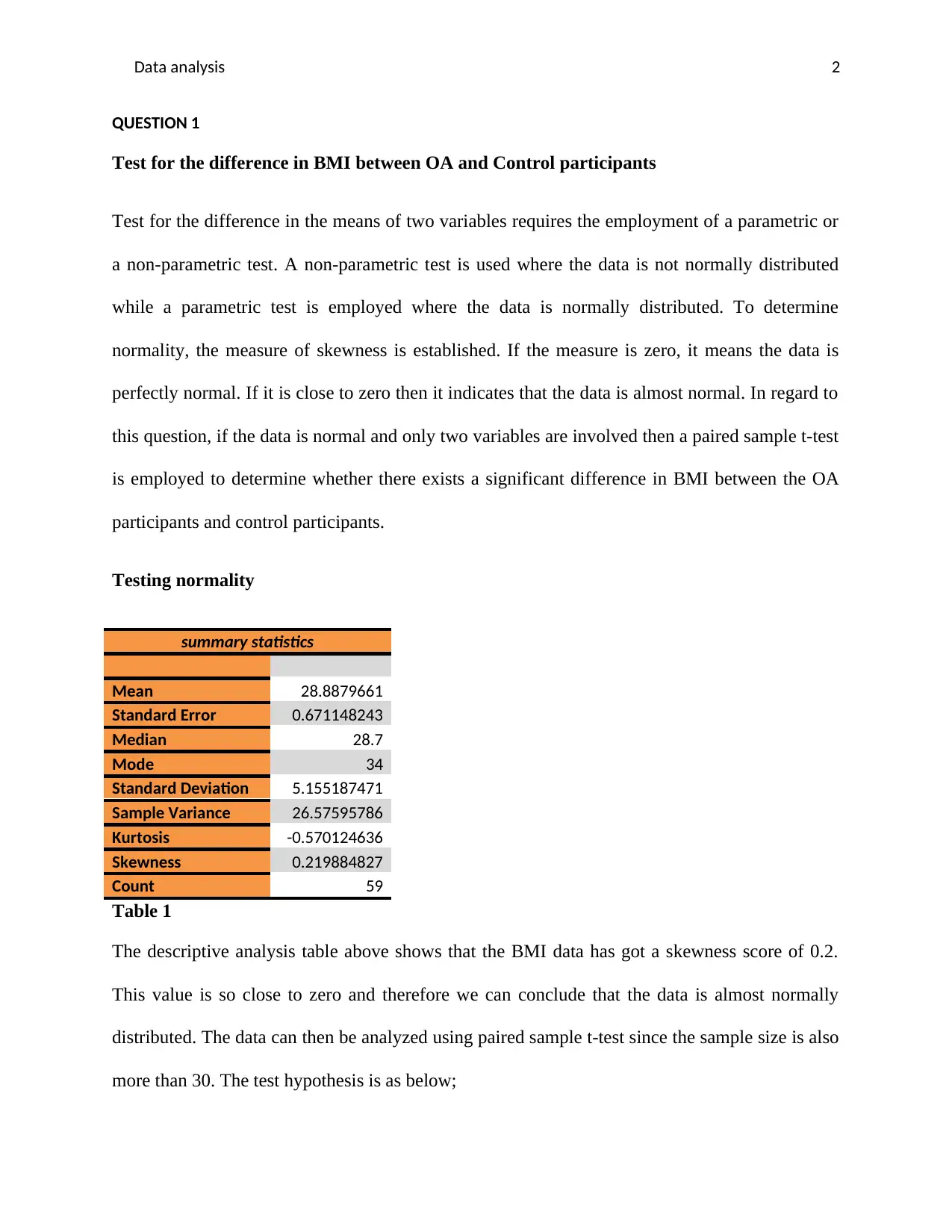
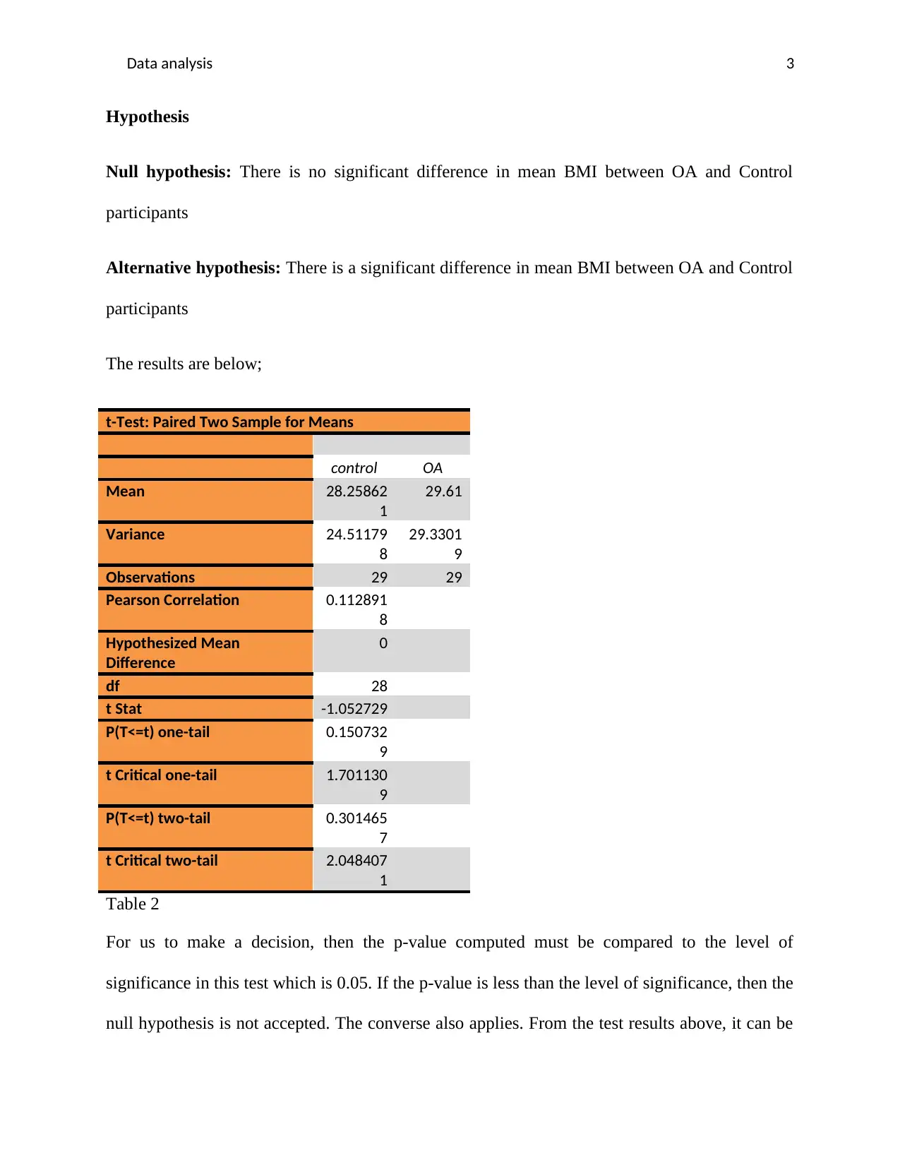
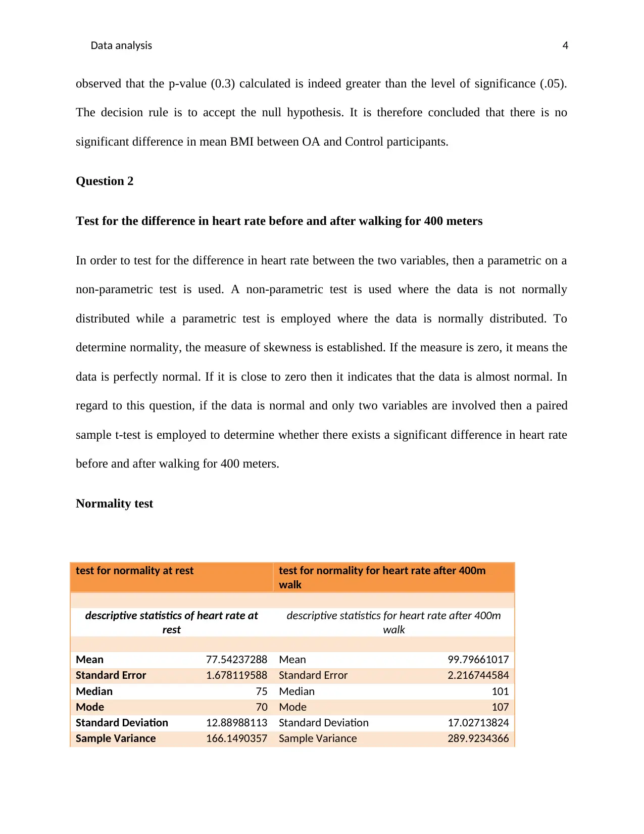
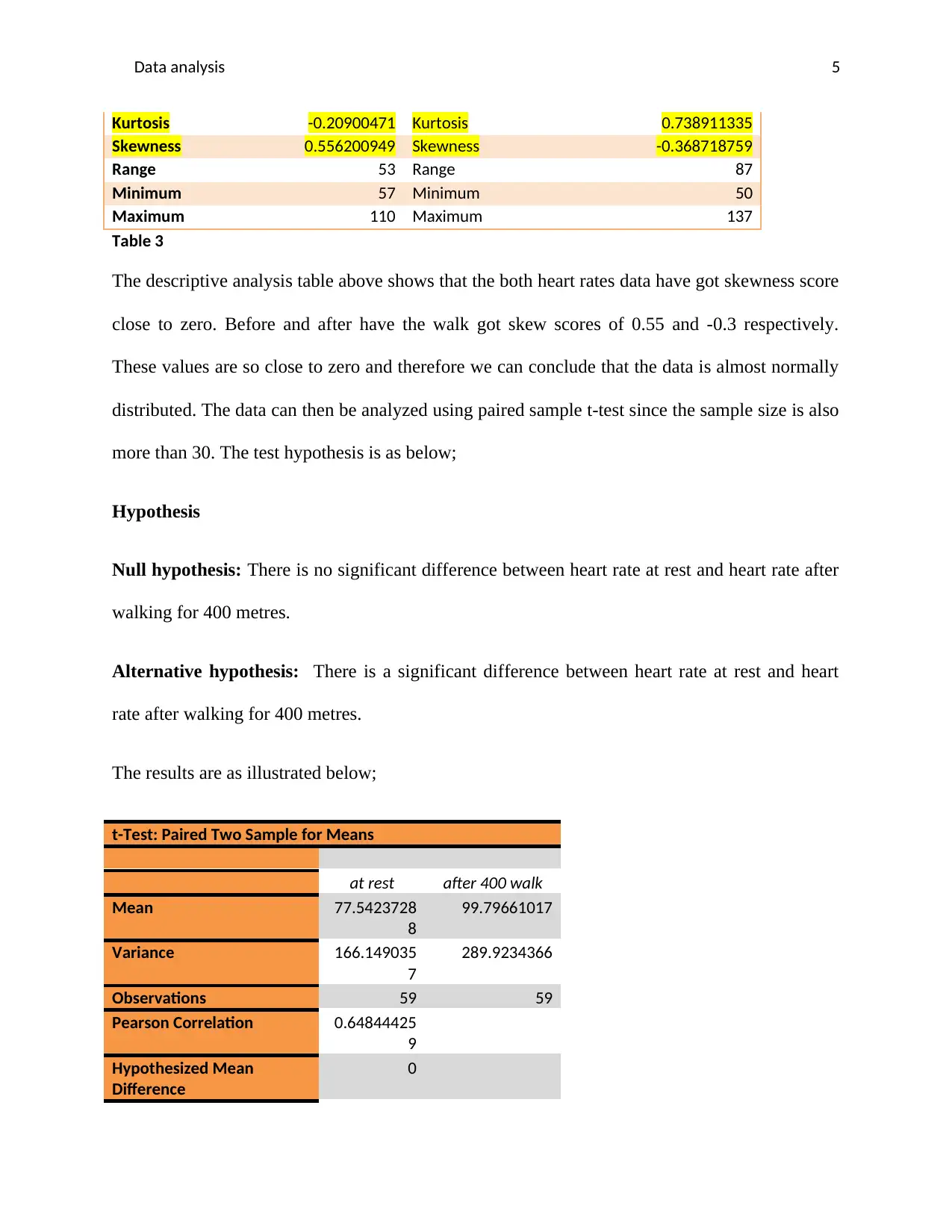
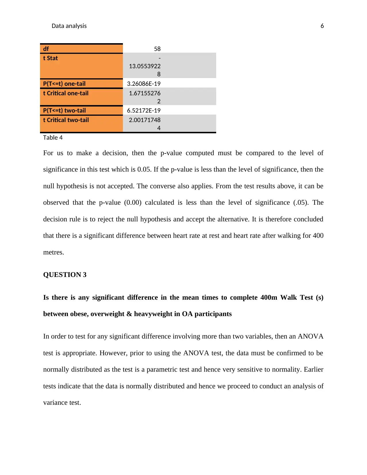
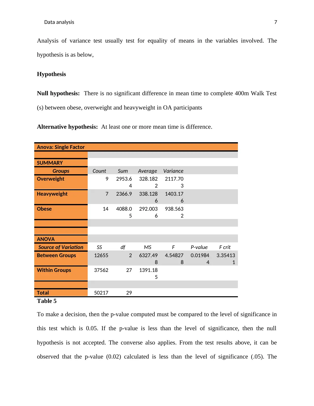
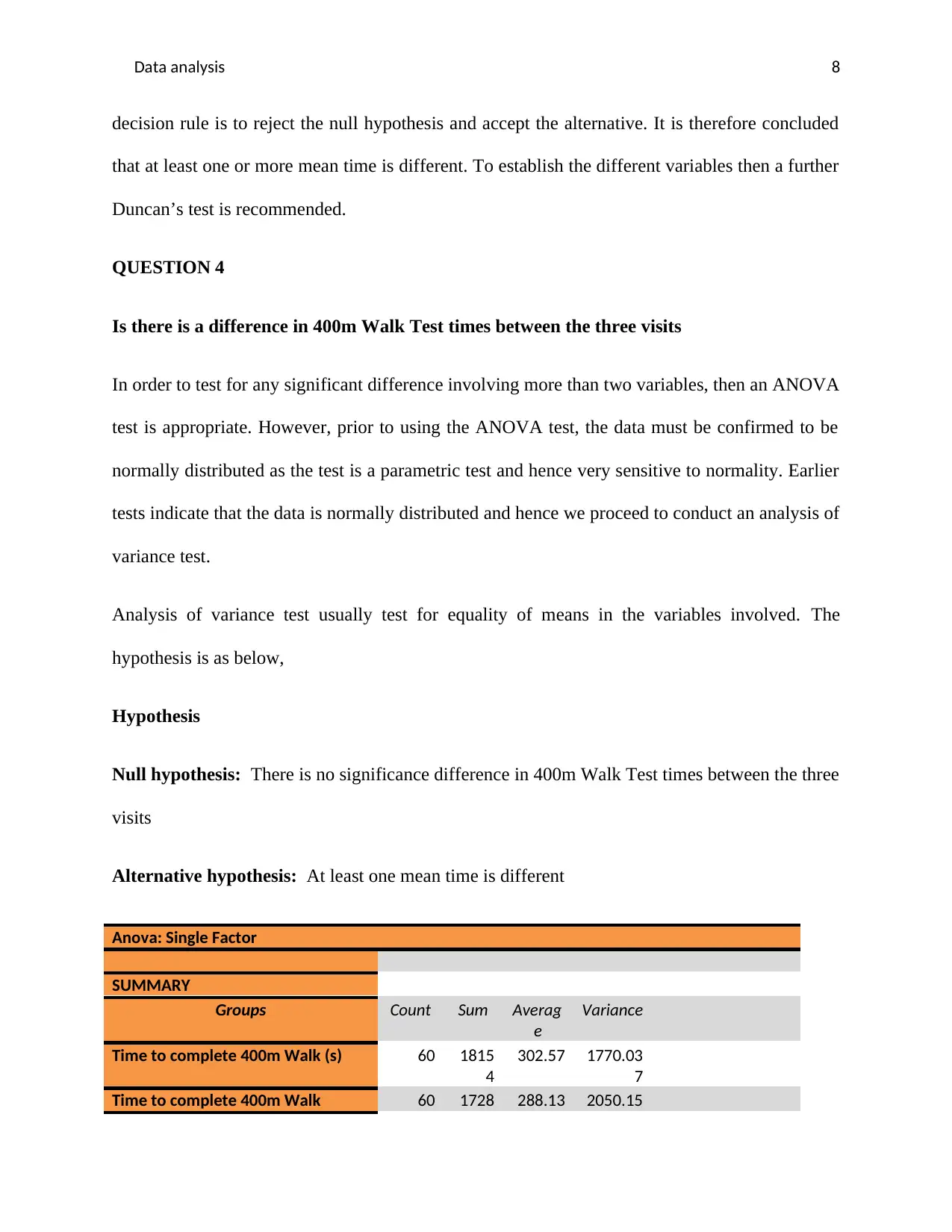
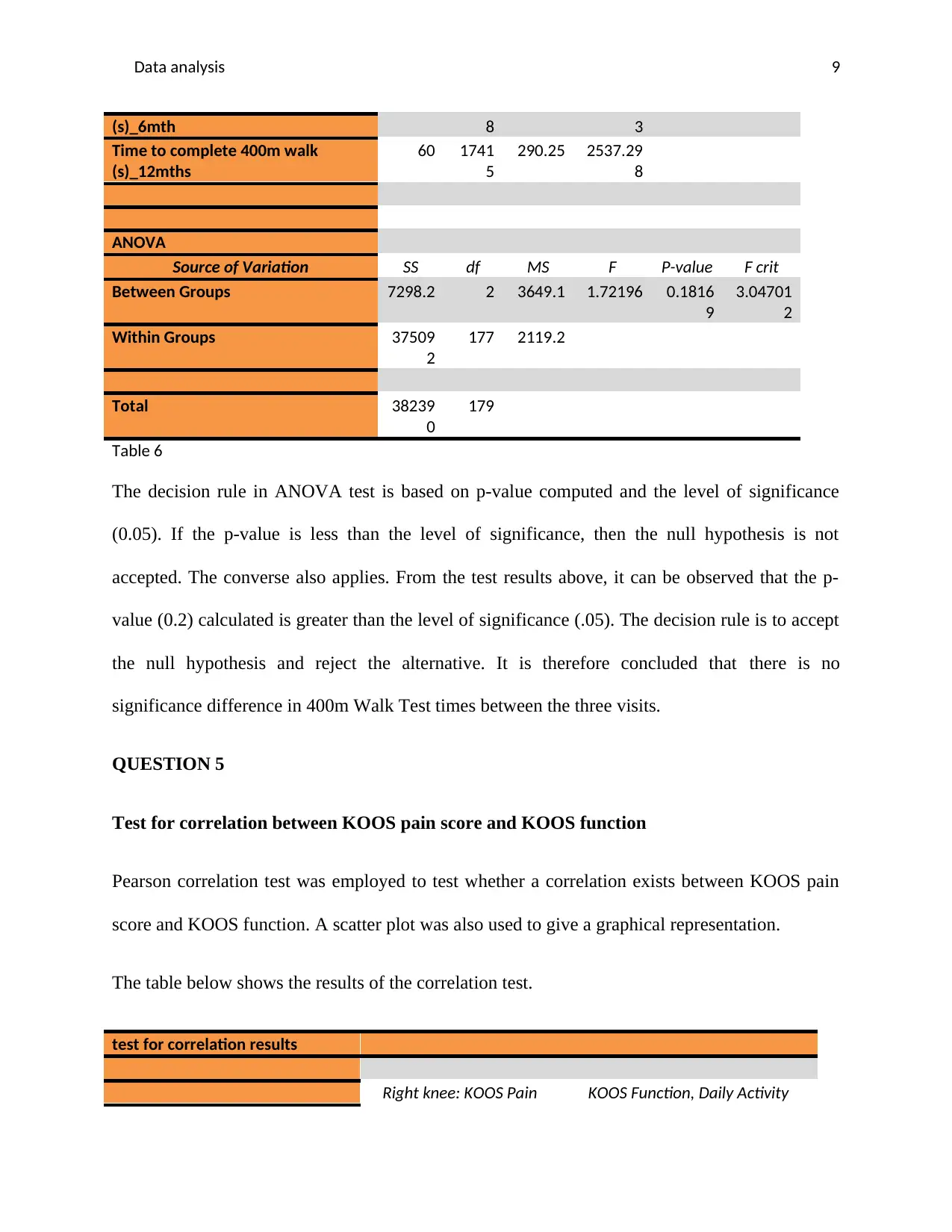
This assignment solution presents a comprehensive analysis of a dataset using various statistical techniques. It begins with an examination of the difference in Body Mass Index (BMI) between Osteoarthritis (OA) and control participants, employing a paired sample t-test after establishing the data's near-normal distribution. The analysis proceeds to assess heart rate changes before and after a 400-meter walk, again utilizing a paired sample t-test to determine significant differences. Furthermore, the solution investigates the impact of weight categories (obese, overweight, heavyweight) on the time to complete a 400-meter walk using ANOVA, and subsequently, the difference in 400m walk test times across three visits. Finally, the assignment explores the correlation between KOOS pain and function scores using a Pearson correlation test and simple regression analysis to determine the relationship between age and the time taken to complete the 400-meter walk. The document provides detailed interpretations of the results, including p-values, and decision rules for each test, offering a complete statistical analysis of the provided data.

Data analysis 1
Student Name:
Student number:
Lecturer:

Data analysis 2
QUESTION 1
Test for the difference in BMI between OA and Control participants
Test for the difference in the means of two variables requires the employment of a parametric or
a non-parametric test. A non-parametric test is used where the data is not normally distributed
while a parametric test is employed where the data is normally distributed. To determine
normality, the measure of skewness is established. If the measure is zero, it means the data is
perfectly normal. If it is close to zero then it indicates that the data is almost normal. In regard to
this question, if the data is normal and only two variables are involved then a paired sample t-test
is employed to determine whether there exists a significant difference in BMI between the OA
participants and control participants.
Testing normality
summary statistics
Mean 28.8879661
Standard Error 0.671148243
Median 28.7
Mode 34
Standard Deviation 5.155187471
Sample Variance 26.57595786
Kurtosis -0.570124636
Skewness 0.219884827
Count 59
Table 1
The descriptive analysis table above shows that the BMI data has got a skewness score of 0.2.
This value is so close to zero and therefore we can conclude that the data is almost normally
distributed. The data can then be analyzed using paired sample t-test since the sample size is also
more than 30. The test hypothesis is as below;

Data analysis 3
Hypothesis
Null hypothesis: There is no significant difference in mean BMI between OA and Control
participants
Alternative hypothesis: There is a significant difference in mean BMI between OA and Control
participants
The results are below;
t-Test: Paired Two Sample for Means
control OA
Mean 28.25862
1
29.61
Variance 24.51179
8
29.3301
9
Observations 29 29
Pearson Correlation 0.112891
8
Hypothesized Mean
Difference
0
df 28
t Stat -1.052729
P(T<=t) one-tail 0.150732
9
t Critical one-tail 1.701130
9
P(T<=t) two-tail 0.301465
7
t Critical two-tail 2.048407
1
Table 2
For us to make a decision, then the p-value computed must be compared to the level of
significance in this test which is 0.05. If the p-value is less than the level of significance, then the
null hypothesis is not accepted. The converse also applies. From the test results above, it can be

Data analysis 4
observed that the p-value (0.3) calculated is indeed greater than the level of significance (.05).
The decision rule is to accept the null hypothesis. It is therefore concluded that there is no
significant difference in mean BMI between OA and Control participants.
Question 2
Test for the difference in heart rate before and after walking for 400 meters
In order to test for the difference in heart rate between the two variables, then a parametric on a
non-parametric test is used. A non-parametric test is used where the data is not normally
distributed while a parametric test is employed where the data is normally distributed. To
determine normality, the measure of skewness is established. If the measure is zero, it means the
data is perfectly normal. If it is close to zero then it indicates that the data is almost normal. In
regard to this question, if the data is normal and only two variables are involved then a paired
sample t-test is employed to determine whether there exists a significant difference in heart rate
before and after walking for 400 meters.
Normality test
test for normality at rest test for normality for heart rate after 400m
walk
descriptive statistics of heart rate at
rest
descriptive statistics for heart rate after 400m
walk
Mean 77.54237288 Mean 99.79661017
Standard Error 1.678119588 Standard Error 2.216744584
Median 75 Median 101
Mode 70 Mode 107
Standard Deviation 12.88988113 Standard Deviation 17.02713824
Sample Variance 166.1490357 Sample Variance 289.9234366

Data analysis 5
Kurtosis -0.20900471 Kurtosis 0.738911335
Skewness 0.556200949 Skewness -0.368718759
Range 53 Range 87
Minimum 57 Minimum 50
Maximum 110 Maximum 137
Table 3
The descriptive analysis table above shows that the both heart rates data have got skewness score
close to zero. Before and after have the walk got skew scores of 0.55 and -0.3 respectively.
These values are so close to zero and therefore we can conclude that the data is almost normally
distributed. The data can then be analyzed using paired sample t-test since the sample size is also
more than 30. The test hypothesis is as below;
Hypothesis
Null hypothesis: There is no significant difference between heart rate at rest and heart rate after
walking for 400 metres.
Alternative hypothesis: There is a significant difference between heart rate at rest and heart
rate after walking for 400 metres.
The results are as illustrated below;
t-Test: Paired Two Sample for Means
at rest after 400 walk
Mean 77.5423728
8
99.79661017
Variance 166.149035
7
289.9234366
Observations 59 59
Pearson Correlation 0.64844425
9
Hypothesized Mean
Difference
0

Data analysis 6
df 58
t Stat -
13.0553922
8
P(T<=t) one-tail 3.26086E-19
t Critical one-tail 1.67155276
2
P(T<=t) two-tail 6.52172E-19
t Critical two-tail 2.00171748
4
Table 4
For us to make a decision, then the p-value computed must be compared to the level of
significance in this test which is 0.05. If the p-value is less than the level of significance, then the
null hypothesis is not accepted. The converse also applies. From the test results above, it can be
observed that the p-value (0.00) calculated is less than the level of significance (.05). The
decision rule is to reject the null hypothesis and accept the alternative. It is therefore concluded
that there is a significant difference between heart rate at rest and heart rate after walking for 400
metres.
QUESTION 3
Is there is any significant difference in the mean times to complete 400m Walk Test (s)
between obese, overweight & heavyweight in OA participants
In order to test for any significant difference involving more than two variables, then an ANOVA
test is appropriate. However, prior to using the ANOVA test, the data must be confirmed to be
normally distributed as the test is a parametric test and hence very sensitive to normality. Earlier
tests indicate that the data is normally distributed and hence we proceed to conduct an analysis of
variance test.

Data analysis 7
Analysis of variance test usually test for equality of means in the variables involved. The
hypothesis is as below,
Hypothesis
Null hypothesis: There is no significant difference in mean time to complete 400m Walk Test
(s) between obese, overweight and heavyweight in OA participants
Alternative hypothesis: At least one or more mean time is difference.
Anova: Single Factor
SUMMARY
Groups Count Sum Average Variance
Overweight 9 2953.6
4
328.182
2
2117.70
3
Heavyweight 7 2366.9 338.128
6
1403.17
6
Obese 14 4088.0
5
292.003
6
938.563
2
ANOVA
Source of Variation SS df MS F P-value F crit
Between Groups 12655 2 6327.49
8
4.54827
8
0.01984
4
3.35413
1
Within Groups 37562 27 1391.18
5
Total 50217 29
Table 5
To make a decision, then the p-value computed must be compared to the level of significance in
this test which is 0.05. If the p-value is less than the level of significance, then the null
hypothesis is not accepted. The converse also applies. From the test results above, it can be
observed that the p-value (0.02) calculated is less than the level of significance (.05). The

Data analysis 8
decision rule is to reject the null hypothesis and accept the alternative. It is therefore concluded
that at least one or more mean time is different. To establish the different variables then a further
Duncan’s test is recommended.
QUESTION 4
Is there is a difference in 400m Walk Test times between the three visits
In order to test for any significant difference involving more than two variables, then an ANOVA
test is appropriate. However, prior to using the ANOVA test, the data must be confirmed to be
normally distributed as the test is a parametric test and hence very sensitive to normality. Earlier
tests indicate that the data is normally distributed and hence we proceed to conduct an analysis of
variance test.
Analysis of variance test usually test for equality of means in the variables involved. The
hypothesis is as below,
Hypothesis
Null hypothesis: There is no significance difference in 400m Walk Test times between the three
visits
Alternative hypothesis: At least one mean time is different
Anova: Single Factor
SUMMARY
Groups Count Sum Averag
e
Variance
Time to complete 400m Walk (s) 60 1815
4
302.57 1770.03
7
Time to complete 400m Walk 60 1728 288.13 2050.15

Data analysis 9
(s)_6mth 8 3
Time to complete 400m walk
(s)_12mths
60 1741
5
290.25 2537.29
8
ANOVA
Source of Variation SS df MS F P-value F crit
Between Groups 7298.2 2 3649.1 1.72196 0.1816
9
3.04701
2
Within Groups 37509
2
177 2119.2
Total 38239
0
179
Table 6
The decision rule in ANOVA test is based on p-value computed and the level of significance
(0.05). If the p-value is less than the level of significance, then the null hypothesis is not
accepted. The converse also applies. From the test results above, it can be observed that the p-
value (0.2) calculated is greater than the level of significance (.05). The decision rule is to accept
the null hypothesis and reject the alternative. It is therefore concluded that there is no
significance difference in 400m Walk Test times between the three visits.
QUESTION 5
Test for correlation between KOOS pain score and KOOS function
Pearson correlation test was employed to test whether a correlation exists between KOOS pain
score and KOOS function. A scatter plot was also used to give a graphical representation.
The table below shows the results of the correlation test.
test for correlation results
Right knee: KOOS Pain KOOS Function, Daily Activity

Data analysis 10
Score
Right knee: KOOS Pain Score 1
KOOS Function, Daily Activity 0.59315549 1
Table 7
Scatterplot diagram
50 60 70 80 90 100 110
0
20
40
60
80
100
120
f(x) = 0.733257215329748 x + 21.111530780905
R² = 0.351833435215427
Scatterplot
KOOS pain score
KOOS function
Figure 1
It can be seen that the Pearson correlation value computed is 0.6. This means that a positive and
significant correlation exists between KOOS pain score and KOOS pain.
QUESTION 6
Simple regression analysis between time taken to complete 400 meters walk and age
Since there is only one independent variable (age), a simple regression analysis is appropriate to
determine whether age can be a better determiner of the time taken to walk the 400 meters. The
regression analysis results are as illustrated in the table below;
SUMMARY
OUTPUT

Data analysis 11
Regression Statistics
Multiple R 0.544139951
R Square 0.296088286
Adjusted R Square 0.283738958
Standard Error 35.75032737
Observations 59
ANOVA
df SS MS F Significance
F
Regression 1 30643.47 30643.47 23.97606 8.41E-06
Residual 57 72850.9 1278.086
Total 58 103494.4
Coefficients Standard
Error
t Stat P-value Lower 95% Upper
95%
Lower
95.0%
Up
95
Intercept 146.6972996 32.06811 4.574555 2.62E-05 82.48203 210.9126 82.48203 210
68 2.516814751 0.513999 4.896536 8.41E-06 1.487549 3.54608 1.487549 3.5
Table 7
40 45 50 55 60 65 70 75 80 85
0
50
100
150
200
250
300
350
400
450
f(x) = 2.53590949483902 x + 145.768262902454
R² = 0.300279999340709
Scatter plot
AGE
Time (s)
Figure 2
It can be observed that the regression analysis above between age and time taken to complete
400 meters walk has R-squared value of 0.3. This means that age as an independent variable can
only explain 30% of the variations in time taken to finish 400 meters walk. The model is

Data analysis 12
therefore not a fit predictor and hence age since it cannot explain 70% of the variation in the
dependent variable, time.