University Assignment: Application of Statistical Theories - FIN 2021
VerifiedAdded on 2022/10/11
|11
|2049
|17
Homework Assignment
AI Summary
This assignment delves into the practical application of statistical theories, primarily focusing on Value at Risk (VaR) as a risk management tool. It explores the advantages and limitations of VaR, detailing its calculation using variance-covariance, historical simulation, and Monte Carlo simulation methods. The assignment also explains the Central Limit Theorem (CLT) and its implications for statistical analysis, including the conditions for its application and the impact of sample size on standard error. A problem-solving section demonstrates the application of these concepts, calculating probabilities based on sample size variations, and the assignment concludes with references to relevant academic sources.
Application of Statistical Theories 1
APPLICATION OF STATISTICAL THEORIES
By Student’s Name
Course Name
Professor’s Name
University Name
City and State
Date
APPLICATION OF STATISTICAL THEORIES
By Student’s Name
Course Name
Professor’s Name
University Name
City and State
Date
Paraphrase This Document
Need a fresh take? Get an instant paraphrase of this document with our AI Paraphraser
Application of Statistical Theories 2
a) VaR
Value at Risk, VaR is a statistical metric which utilizes the normal distribution
knowledge to estimate the expected minimum loss of value a company with a given probability
for a specific period (Hartmann, 2016). VaR is widely utilized in the financial industry for
budgeting and risk mitigation purposes. The risk management statistical concept introduced in
the 1980s has many advantages.
The major advantage of VaR is its wide application in the financial industry. The
application of VaR statistical concept for risk estimation is not limited to any industry. VaR is a
standard metric applicable across various industries in an attempt to estimates the potential
financial risk exposure for institutions, companies, and parastatals (Davies, 2017; Zax, 2011).
Moreover, VaR calculation is easy; therefore, managers, senior managers, and company's
directors who are not experts in statistics easily understand and interpret the concept. Besides the
minimum loss of value estimation, VaR is a very useful tool in risk budgeting and capital
allocation factoring the minimum expected loss of value for every business units in a company or
institution. Hochkirchen (2011) highlighted VaR as a very important tool for risk budgeting and
capital allocation for different business units in cases where a company utilizes a central process
of capital allocation.
Even though VaR has many advantages and wide application, it has a weakness in its
application. VaR measure of risk estimates the minimum loss of value but does not estimate the
expected maximum loss of value in the risk estimation process (The Financial Applications of
Mathematical Statistics, 2014). Estimating the maximum expected loss of value enables the
managers of companies to factor in the resultant financial loss from company activities.
Practically, VaR measure of risk underestimates the frequency and magnitude of losses resulting
Application of Statistical Theories 3
from the assumptions made during VaR calculation. Additionally, VaR utilizes historical data to
predict expected losses in the future. Past data may not be a good predictor of futures events,
especially for black-swan events. Moreover, VaR assumes that the distribution of returns is
normally distributed and follow a bell-shaped graph. Normality assumption is only applicable for
periods of normal market conditions but abnormal market conditions.
VaR Calculation
VaR is measured using three different approaches; the historical simulation, Monte Carlo
simulation, and variance-covariance method. The variance-covariance VaR measure of risk
assumes that the portfolio values follow the normal distribution. The normal distribution is
motivated by the famous central limit theorem. Therefore, a randomly sampled portfolio data is
independent and identical regardless of the distribution of data sample, thus normally distributed
(Notz, 2012). Variance-variance VaR method calculates the standard deviation of price
movements of a security. The calculated expected value (Mean) and the standard deviation
values are used to plot a normal distribution curve against actual data.
⊘ This is a preview!⊘
Do you want full access?
Subscribe today to unlock all pages.
Trusted by 1+ million students worldwide
Application of Statistical Theories 4
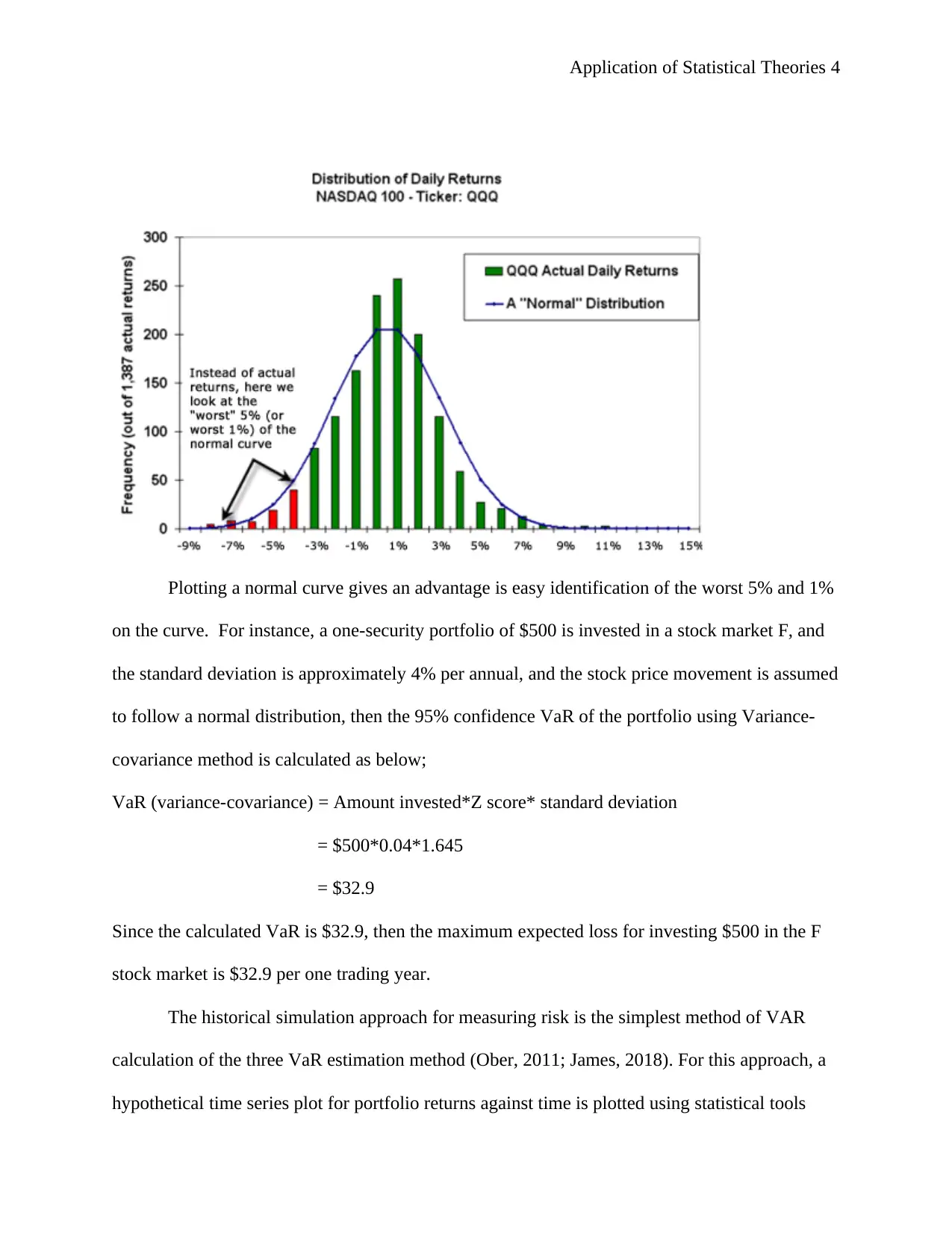
Plotting a normal curve gives an advantage is easy identification of the worst 5% and 1%
on the curve. For instance, a one-security portfolio of $500 is invested in a stock market F, and
the standard deviation is approximately 4% per annual, and the stock price movement is assumed
to follow a normal distribution, then the 95% confidence VaR of the portfolio using Variance-
covariance method is calculated as below;
VaR (variance-covariance) = Amount invested*Z score* standard deviation
= $500*0.04*1.645
= $32.9
Since the calculated VaR is $32.9, then the maximum expected loss for investing $500 in the F
stock market is $32.9 per one trading year.
The historical simulation approach for measuring risk is the simplest method of VAR
calculation of the three VaR estimation method (Ober, 2011; James, 2018). For this approach, a
hypothetical time series plot for portfolio returns against time is plotted using statistical tools
Paraphrase This Document
Need a fresh take? Get an instant paraphrase of this document with our AI Paraphraser
Application of Statistical Theories 5
such as STATA then the change in portfolio returns is plotted for each period. By plotting the
time series,
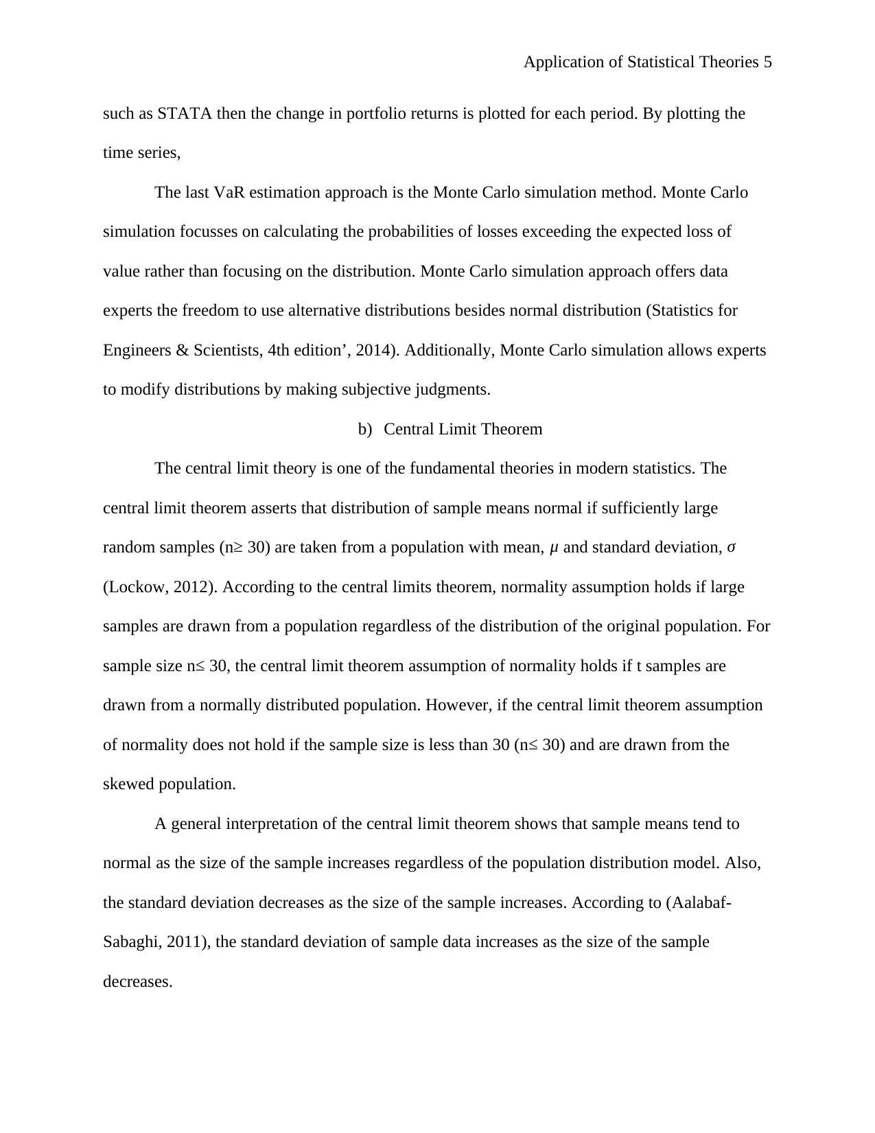
The last VaR estimation approach is the Monte Carlo simulation method. Monte Carlo
simulation focusses on calculating the probabilities of losses exceeding the expected loss of
value rather than focusing on the distribution. Monte Carlo simulation approach offers data
experts the freedom to use alternative distributions besides normal distribution (Statistics for
Engineers & Scientists, 4th edition’, 2014). Additionally, Monte Carlo simulation allows experts
to modify distributions by making subjective judgments.
b) Central Limit Theorem
The central limit theory is one of the fundamental theories in modern statistics. The
central limit theorem asserts that distribution of sample means normal if sufficiently large
random samples (n≥ 30) are taken from a population with mean, μ and standard deviation, σ
(Lockow, 2012). According to the central limits theorem, normality assumption holds if large
samples are drawn from a population regardless of the distribution of the original population. For
sample size n ≤ 30, the central limit theorem assumption of normality holds if t samples are
drawn from a normally distributed population. However, if the central limit theorem assumption
of normality does not hold if the sample size is less than 30 (n≤ 30) and are drawn from the
skewed population.
A general interpretation of the central limit theorem shows that sample means tend to
normal as the size of the sample increases regardless of the population distribution model. Also,
the standard deviation decreases as the size of the sample increases. According to (Aalabaf-
Sabaghi, 2011), the standard deviation of sample data increases as the size of the sample
decreases.
such as STATA then the change in portfolio returns is plotted for each period. By plotting the
time series,
The last VaR estimation approach is the Monte Carlo simulation method. Monte Carlo
simulation focusses on calculating the probabilities of losses exceeding the expected loss of
value rather than focusing on the distribution. Monte Carlo simulation approach offers data
experts the freedom to use alternative distributions besides normal distribution (Statistics for
Engineers & Scientists, 4th edition’, 2014). Additionally, Monte Carlo simulation allows experts
to modify distributions by making subjective judgments.
b) Central Limit Theorem
The central limit theory is one of the fundamental theories in modern statistics. The
central limit theorem asserts that distribution of sample means normal if sufficiently large
random samples (n≥ 30) are taken from a population with mean, μ and standard deviation, σ
(Lockow, 2012). According to the central limits theorem, normality assumption holds if large
samples are drawn from a population regardless of the distribution of the original population. For
sample size n ≤ 30, the central limit theorem assumption of normality holds if t samples are
drawn from a normally distributed population. However, if the central limit theorem assumption
of normality does not hold if the sample size is less than 30 (n≤ 30) and are drawn from the
skewed population.
A general interpretation of the central limit theorem shows that sample means tend to
normal as the size of the sample increases regardless of the population distribution model. Also,
the standard deviation decreases as the size of the sample increases. According to (Aalabaf-
Sabaghi, 2011), the standard deviation of sample data increases as the size of the sample
decreases.
Application of Statistical Theories 6
The application of central limit theorem is restricted to three conditions. One of the
conditions for independence of samples and sufficiently large sample size or follow a population
distribution. The second condition for independent and identically distributed random variables
is the 10% rule. The 10% rule asserts that the sample size must be less or equal to 10% of the
population size. Lastly, the size of the sample must be large enough such that np≥10 and nq≥10.
The application of the “10% Rule”, randomization condition, and sample size condition is vital
for accurate and appropriate application of the central limit theorem (Behara, and BarCharts,
2014).
Random variables X1, X2, …. X n form a random sample of size n if and only if:
i) the Xi s are independent random variables and
ii) every Xi has the same probability distribution
If the above two conditions are satisfied, then the Xis are said to be independent and identically
distributed (Carver, 2017).
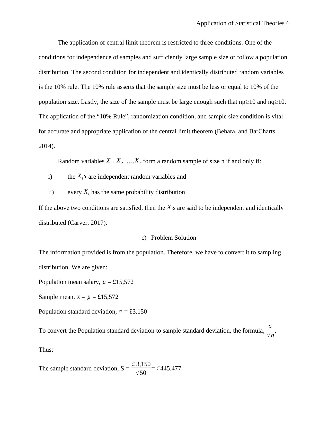
c) Problem Solution
The information provided is from the population. Therefore, we have to convert it to sampling
distribution. We are given:
Population mean salary, μ = £15,572
Sample mean, x = μ = £15,572
Population standard deviation, σ = £3,150
To convert the Population standard deviation to sample standard deviation, the formula, σ
√ n.
Thus;
The sample standard deviation, S = £ 3,150
√50 = £445.477
The application of central limit theorem is restricted to three conditions. One of the
conditions for independence of samples and sufficiently large sample size or follow a population
distribution. The second condition for independent and identically distributed random variables
is the 10% rule. The 10% rule asserts that the sample size must be less or equal to 10% of the
population size. Lastly, the size of the sample must be large enough such that np≥10 and nq≥10.
The application of the “10% Rule”, randomization condition, and sample size condition is vital
for accurate and appropriate application of the central limit theorem (Behara, and BarCharts,
2014).
Random variables X1, X2, …. X n form a random sample of size n if and only if:
i) the Xi s are independent random variables and
ii) every Xi has the same probability distribution
If the above two conditions are satisfied, then the Xis are said to be independent and identically
distributed (Carver, 2017).
c) Problem Solution
The information provided is from the population. Therefore, we have to convert it to sampling
distribution. We are given:
Population mean salary, μ = £15,572
Sample mean, x = μ = £15,572
Population standard deviation, σ = £3,150
To convert the Population standard deviation to sample standard deviation, the formula, σ
√ n.
Thus;
The sample standard deviation, S = £ 3,150
√50 = £445.477
⊘ This is a preview!⊘
Do you want full access?
Subscribe today to unlock all pages.
Trusted by 1+ million students worldwide
Application of Statistical Theories 7
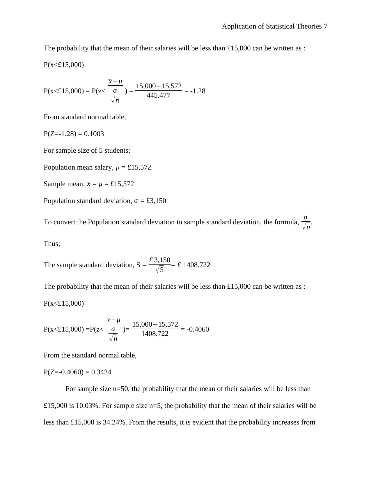
The probability that the mean of their salaries will be less than £15,000 can be written as :
P(x<£15,000)
P(x<£15,000) = P(z<
x−μ
σ
√ n
) = 15,000−15,572
445.477 = -1.28
From standard normal table,
P(Z=-1.28) = 0.1003
For sample size of 5 students;
Population mean salary, μ = £15,572
Sample mean, x = μ = £15,572
Population standard deviation, σ = £3,150
To convert the Population standard deviation to sample standard deviation, the formula, σ
√ n.
Thus;
The sample standard deviation, S = £ 3,150
√5 = £ 1408.722
The probability that the mean of their salaries will be less than £15,000 can be written as :
P(x<£15,000)
P(x<£15,000) =P(z<
x−μ
σ
√n
)= 15,000−15,572
1408.722 = -0.4060
From the standard normal table,
P(Z=-0.4060) = 0.3424
For sample size n=50, the probability that the mean of their salaries will be less than
£15,000 is 10.03%. For sample size n=5, the probability that the mean of their salaries will be
less than £15,000 is 34.24%. From the results, it is evident that the probability increases from
The probability that the mean of their salaries will be less than £15,000 can be written as :
P(x<£15,000)
P(x<£15,000) = P(z<
x−μ
σ
√ n
) = 15,000−15,572
445.477 = -1.28
From standard normal table,
P(Z=-1.28) = 0.1003
For sample size of 5 students;
Population mean salary, μ = £15,572
Sample mean, x = μ = £15,572
Population standard deviation, σ = £3,150
To convert the Population standard deviation to sample standard deviation, the formula, σ
√ n.
Thus;
The sample standard deviation, S = £ 3,150
√5 = £ 1408.722
The probability that the mean of their salaries will be less than £15,000 can be written as :
P(x<£15,000)
P(x<£15,000) =P(z<
x−μ
σ
√n
)= 15,000−15,572
1408.722 = -0.4060
From the standard normal table,
P(Z=-0.4060) = 0.3424
For sample size n=50, the probability that the mean of their salaries will be less than
£15,000 is 10.03%. For sample size n=5, the probability that the mean of their salaries will be
less than £15,000 is 34.24%. From the results, it is evident that the probability increases from
Paraphrase This Document
Need a fresh take? Get an instant paraphrase of this document with our AI Paraphraser
Application of Statistical Theories 8
10.03% to 34.24% by decreasing the sample size from 50 to 5. Therefore, we can conclude that
decreasing the sample size increases the standard error.
References
‘Statistics for Engineers & Scientists, 4th edition’ (2014) Environmental Progress &
Sustainable Energy, 33(3), pp. 667–668. doi: 10.1002/ep.12008.
Aalabaf-Sabaghi, M. (2011) ‘Applied Statistics for Business and Economics’, Journal of
the Royal Statistical Society: Series A (Statistics in Society), 174(3), p. 848. doi:
10.1111/j.1467-985X.2011.00709_11.x.
Behara, R. and BarCharts, I. (2014) Business Statistics. [Boca Raton, FL]: QuickStudy
Reference Guides (Quick Study Business). Available at:
http://search.ebscohost.com/login.aspx?
direct=true&db=nlebk&AN=1534295&site=ehost-live (Accessed: 6 August 2019).
Carver, R. H. (2017) ‘What’s Missing in Intro Stats? Missing Data’, Proceedings for the
Northeast Region Decision Sciences Institute (NEDSI), pp. 786–797. Available at:
http://search.ebscohost.com/login.aspx?
direct=true&db=bth&AN=122933180&site=ehost-live (Accessed: 6 August 2019).
Davies, A. (2017), Understanding Statistics : An Introduction, Libertarianism.org Press,
Washington, D.C., viewed 6 August 2019, <http://search.ebscohost.com/login.aspx?
direct=true&db=nlebk&AN=1667844&site=ehost-live>.
Hartmann, H. (2016) ‘Statistics for Engineers’, Communications of the ACM, 59(7), pp.
58–66. doi: 10.1145/2890780.
Application of Statistical Theories 9
Hochkirchen, T. (2011) ‘Applied Statistics for Engineers and Physical
Scientists’, Journal of the Royal Statistical Society: Series A (Statistics in Society),
174(3), pp. 847–848. doi: 10.1111/j.1467-985X.2011.00709_10.x.
James, G. M. (2018) ‘Statistics within business in the era of big data’, Statistics &
Probability Letters, 136, pp. 155–159. doi: 10.1016/j.spl.2018.02.034.
Lockow, E. (2012) ‘S. J. Morrison: Statistics for Engineers: an introduction’, Statistical
Papers, 53(1), pp. 245–246. doi: 10.1007/s00362-010-0358-x.
Notz, W. (2012) ‘Statistical Engineering, a Missing Ingredient in the Introductory
Statistics Course’, Quality Engineering, 24(2), pp. 193–200. doi:
10.1080/08982112.2012.641145.
Ober, P. (2011) ‘Random Phenomena: Fundamentals of Probability and Statistics for
Engineers’, Journal of Applied Statistics, 38(12), pp. 2989–2990. doi:
10.1080/02664763.2011.559372.
The Financial Applications of Mathematical Statistics (2014). Ipswich, Massachusetts:
Salem Press (Business Reference Guide). Available at:
http://search.ebscohost.com/login.aspx?direct=true&db=nlebk&AN=777879&site=ehost-
live (Accessed: 6 August 2019).
Zax, J. S. (2011) Introductory Econometrics : Intuition, Proof, and Practice. Stanford,
Calif: Stanford Economics and Finance. Available at:
http://search.ebscohost.com/login.aspx?direct=true&db=nlebk&AN=362850&site=ehost-
live (Accessed: 6 August 2019).
⊘ This is a preview!⊘
Do you want full access?
Subscribe today to unlock all pages.
Trusted by 1+ million students worldwide

Application of Statistical Theories 10
Paraphrase This Document
Need a fresh take? Get an instant paraphrase of this document with our AI Paraphraser

Application of Statistical Theories 11
1 out of 11
Related Documents


Your All-in-One AI-Powered Toolkit for Academic Success.
+13062052269
info@desklib.com
Available 24*7 on WhatsApp / Email
![[object Object]](/_next/static/media/star-bottom.7253800d.svg)
Unlock your academic potential
Copyright © 2020–2026 A2Z Services. All Rights Reserved. Developed and managed by ZUCOL.