Report on Statistical Modeling of Gender Wage Gap and Occupation

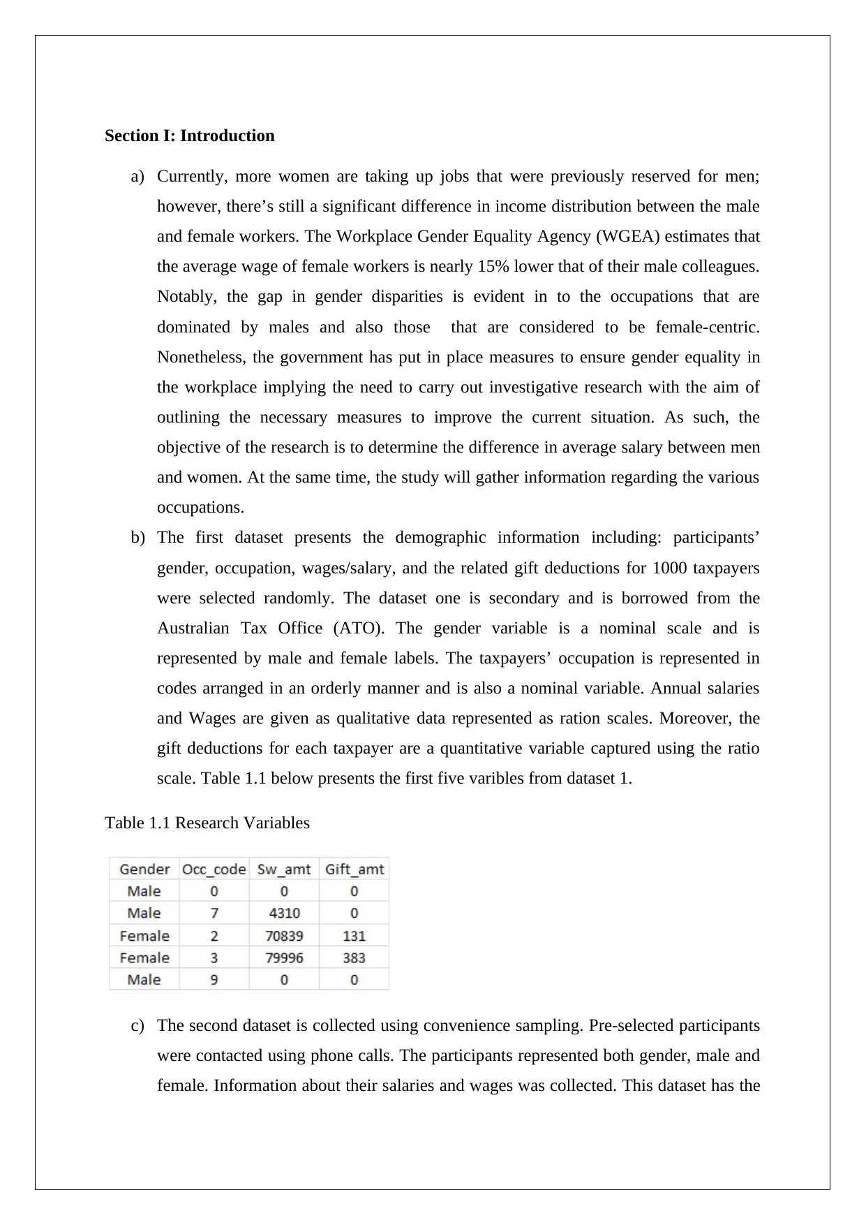
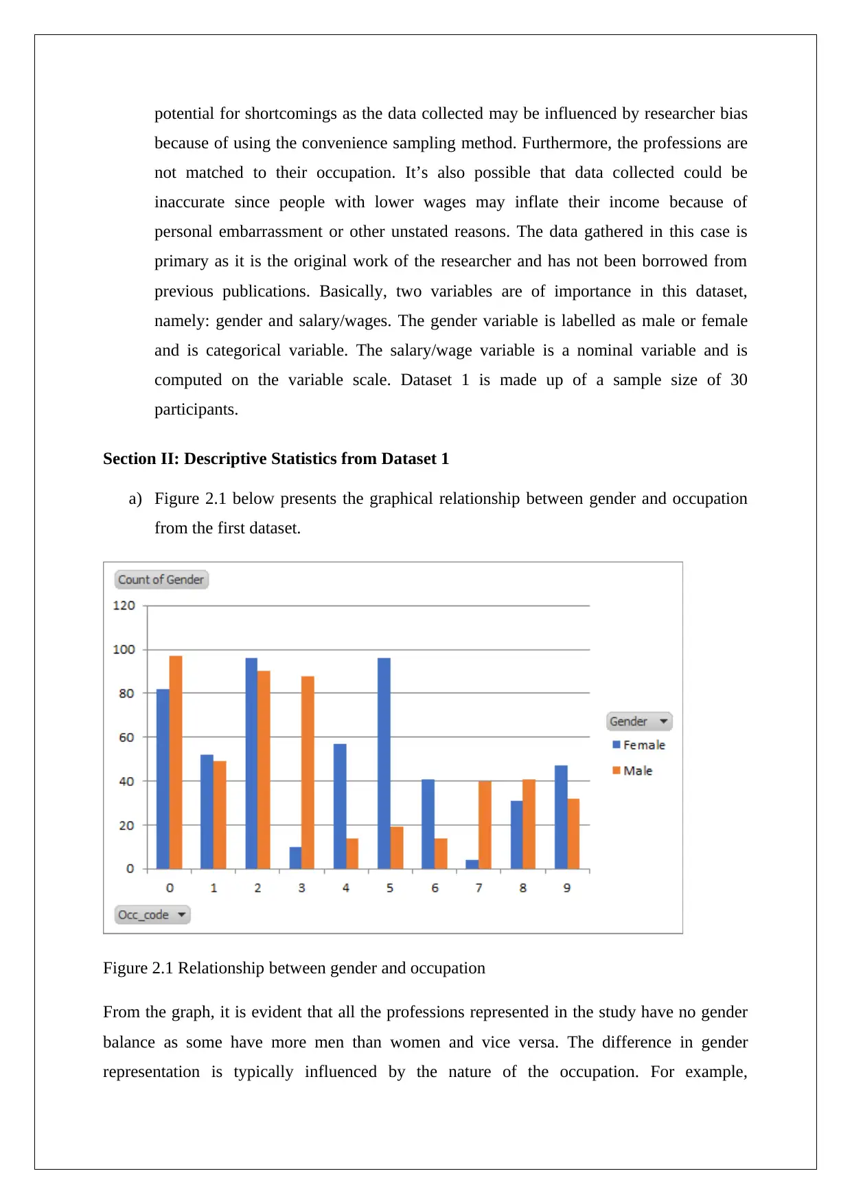
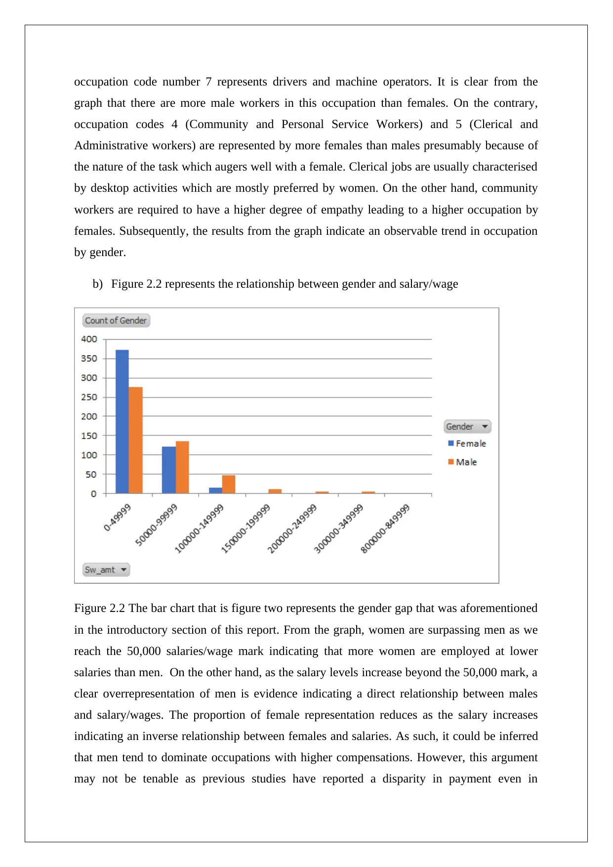
This report presents a statistical analysis of the gender wage gap, examining income disparities between men and women across various occupations. The study utilizes two datasets: one from the Australian Tax Office and another collected through convenience sampling. Descriptive statistics, including graphical representations and numerical summaries, reveal differences in gender representation across different professions and a clear wage gap, with women overrepresented in lower salary brackets. Inferential statistics, such as confidence intervals and t-tests, are used to analyze the data further. The results indicate that there is a significant difference in average income between males and females, and the study finds a significant difference in the average income of males and females. The report concludes that the wage gap is influenced by the distribution of genders in high-paying occupations and recommends further research to understand wage disparities in female-dominated professions. The study uses t-test analysis and hypothesis testing to determine the gender gap in the average income and finds that the difference in the average income of males and females is not significant.

STATISTICAL MODELLING
STUDENT ID:
[Pick the date]

Section I: Introduction
a) Currently, more women are taking up jobs that were previously reserved for men;
however, there’s still a significant difference in income distribution between the male
and female workers. The Workplace Gender Equality Agency (WGEA) estimates that
the average wage of female workers is nearly 15% lower that of their male colleagues.
Notably, the gap in gender disparities is evident in to the occupations that are
dominated by males and also those that are considered to be female-centric.
Nonetheless, the government has put in place measures to ensure gender equality in
the workplace implying the need to carry out investigative research with the aim of
outlining the necessary measures to improve the current situation. As such, the
objective of the research is to determine the difference in average salary between men
and women. At the same time, the study will gather information regarding the various
occupations.
b) The first dataset presents the demographic information including: participants’
gender, occupation, wages/salary, and the related gift deductions for 1000 taxpayers
were selected randomly. The dataset one is secondary and is borrowed from the
Australian Tax Office (ATO). The gender variable is a nominal scale and is
represented by male and female labels. The taxpayers’ occupation is represented in
codes arranged in an orderly manner and is also a nominal variable. Annual salaries
and Wages are given as qualitative data represented as ration scales. Moreover, the
gift deductions for each taxpayer are a quantitative variable captured using the ratio
scale. Table 1.1 below presents the first five varibles from dataset 1.
Table 1.1 Research Variables
c) The second dataset is collected using convenience sampling. Pre-selected participants
were contacted using phone calls. The participants represented both gender, male and
female. Information about their salaries and wages was collected. This dataset has the

potential for shortcomings as the data collected may be influenced by researcher bias
because of using the convenience sampling method. Furthermore, the professions are
not matched to their occupation. It’s also possible that data collected could be
inaccurate since people with lower wages may inflate their income because of
personal embarrassment or other unstated reasons. The data gathered in this case is
primary as it is the original work of the researcher and has not been borrowed from
previous publications. Basically, two variables are of importance in this dataset,
namely: gender and salary/wages. The gender variable is labelled as male or female
and is categorical variable. The salary/wage variable is a nominal variable and is
computed on the variable scale. Dataset 1 is made up of a sample size of 30
participants.
Section II: Descriptive Statistics from Dataset 1
a) Figure 2.1 below presents the graphical relationship between gender and occupation
from the first dataset.
Figure 2.1 Relationship between gender and occupation
From the graph, it is evident that all the professions represented in the study have no gender
balance as some have more men than women and vice versa. The difference in gender
representation is typically influenced by the nature of the occupation. For example,

occupation code number 7 represents drivers and machine operators. It is clear from the
graph that there are more male workers in this occupation than females. On the contrary,
occupation codes 4 (Community and Personal Service Workers) and 5 (Clerical and
Administrative workers) are represented by more females than males presumably because of
the nature of the task which augers well with a female. Clerical jobs are usually characterised
by desktop activities which are mostly preferred by women. On the other hand, community
workers are required to have a higher degree of empathy leading to a higher occupation by
females. Subsequently, the results from the graph indicate an observable trend in occupation
by gender.
b) Figure 2.2 represents the relationship between gender and salary/wage
Figure 2.2 The bar chart that is figure two represents the gender gap that was aforementioned
in the introductory section of this report. From the graph, women are surpassing men as we
reach the 50,000 salaries/wage mark indicating that more women are employed at lower
salaries than men. On the other hand, as the salary levels increase beyond the 50,000 mark, a
clear overrepresentation of men is evidence indicating a direct relationship between males
and salary/wages. The proportion of female representation reduces as the salary increases
indicating an inverse relationship between females and salaries. As such, it could be inferred
that men tend to dominate occupations with higher compensations. However, this argument
may not be tenable as previous studies have reported a disparity in payment even in

occupations that are presumed to be female-centric. The graph is, therefore, an indicator of
the disconnected compensation between male and female genders.
c) Table 2.1 below represents the numerical summary of gender and compensation
Table 2.1: Relationship between gender and compensation
Interestingly, although females represent the most significant percentage, they also represent
the largest sample with the lowest compensation, that is, 50,000 and below. Concurrently, the
representation of females is lower in all the other salary levels as the amount of compensation
increases. The table is a clear indicator of the dismal representation of females in the high
paying jobs possibly implying a window ceiling below which women must choose an inferior
administrative position. While the observed pattern in compensation disparity is attributed to
the distribution of the occupation among the genders, the entire difference cannot be solely
attributed to the occupation profile.
d) Figure 2.3 below presents the relationship between income and deduction gifts

Figure 2.3: Relationship between income and deduction gifts
From the scatter plot that is figure 3 shows no significant relationship between the existing
variables. These findings are emphasised by the R2 computation that is almost zero, implying
a non-significant correlation between the variables. Nonetheless, the observed outcome is an
expected trend since it is not fundamental that employees who are earning a higher income
would give an equally higher donation. The donation is dependent on the taxpayer’s
orientation which does not necessarily share a significant correlation with the level of income
as illustrated by the scatter plot in figure 3.
Section II: Inferential Statistics
a) The result shows the income levels for various professions. The data is classified
according to the code of occupation and computed the median income level.
Accordingly, the occupation codes with the highest median income level are 1, 2, 3,
and 5.
The 95% coefficient interval of the sample levels of participation regarding the data
provided was used to estimate the gender representatives in the sample population. Table 3.1
below shows the computation of the requisite confidence intervals for the profession.
Table 3.1: Occupation Code 1

From the results in figure 3.1, it can be inferred that with 95% confidence the number
of female in code one occupation would vary between 0.4174 and 0.6123.
Table 3.2: Occupation Code 3
From the results in table 3.2, it can be inferred that with the 95% confidence level, the
number of females in code three occupation varies between 0.0421 and 0.1620.
Table 3.3: Occupation Code 2
From the results in table 3.3, it can be concluded that at 95% confidence level the
number of female workers in code two occupation varies between 0.4443 and 0.5879.

Table 3.4 Occupation Code 5
According to the data in figure 3.4 at the 95% confidence interval, the number of
occupying positions in job code 5 varies between 0.7669 and 0.9027.
According to the findings, the estimated occupation by females in high paying
professions is very low. There is only one female occupying the top four occupations where
the job at hand involves managing a majority proportion.
b) The test hypothesis are:
Null Hypothesis, H0: p≤0.8; that is, percentage of males who drive and operate
machines is not more than 80% or 0.8.
Alternative Hypothesis, H1: p>0.8; that is, percentage of males driving or operating
machines exceeds 80% or 0.8.
The necessary computations according to the hypotheses are illustrated in table 3.5
below.
Table 3.5: Occupation Code 7

The above computation shows a p-value of 0.0440 and the significance level of the
hypothesis is 5%. With the p-value being <5%, there is enough evidence to reject the null
hypothesis and support the alternative hypothesis. Therefore, in conclusion, the number of
males in occupation code 7 is higher than 90% of the sample of both genders with less 10%
being occupied by their female counterparts.
c) The test hypotheses are:
H0: μfemale = μmale, that is, there is no significant difference in the average income for
males and females
H1: μfemale ≠ μmale, that is, there is a significant difference in the average income of
males and females
The t-test analysis will be utilised in computation of the data being that the standard
deviation is unknown. The results of the analysis are presented in table 3.6 below.

Table 3.6: T-test results
The test is two-tail, thence; the p-value would be useful. From table 3.6, the outcome
of the p-value is zero. The test reveals a significance level of 5 % for the hypothesis. Since
the P-value < 5 %, the research has sufficient evidence to reject the null hypothesis and
accept the alternative hypothesis. Therefore, the study concludes that a significant difference
exists in the income averages of both males and females.
d) Hypotheses to determine the gender gap in the average income
H0: μfemale = μmale
H1: μfemale ≠ μmale
The t-test analysis is used to test the hypotheses because the standard deviation is not
known. The output of the t-test analysis is presented in table 3.7 below.

Table 3.7: T-test
From table 3.7 the two-tail p-value is 0.4889 which is higher than the 0.09 %
significance level. Therefore, the study cannot reject the null hypothesis (μfemale = μmale). The
study thus concludes that the difference in the average income of males and females is not
significant.
Section 4: Conclusion
a) In conclusion, there is a gap between the male and female genders. One of the
primary reasons behind the observed disparity between male and female income
levels in the existing trend whereby more men than women occupy the professions
with a higher median income. On the contrary, the study finds no significant
relationship between annual income levels and gift deduction amounts which are
influenced by personal incentives rather than income levels. At the same time, the
gender representations vary across the different occupations studied under this
research.
b) The study recommends further research to consider investigating the reasons for the
observed wage disparity in occupations where females form the majority proportion.
It is imperative that the observed wage difference between males and females be
because there are more males than females occupying the professions with a higher
median income.