Statistics 630 - Assignment 8: Probability & Statistics Solutions

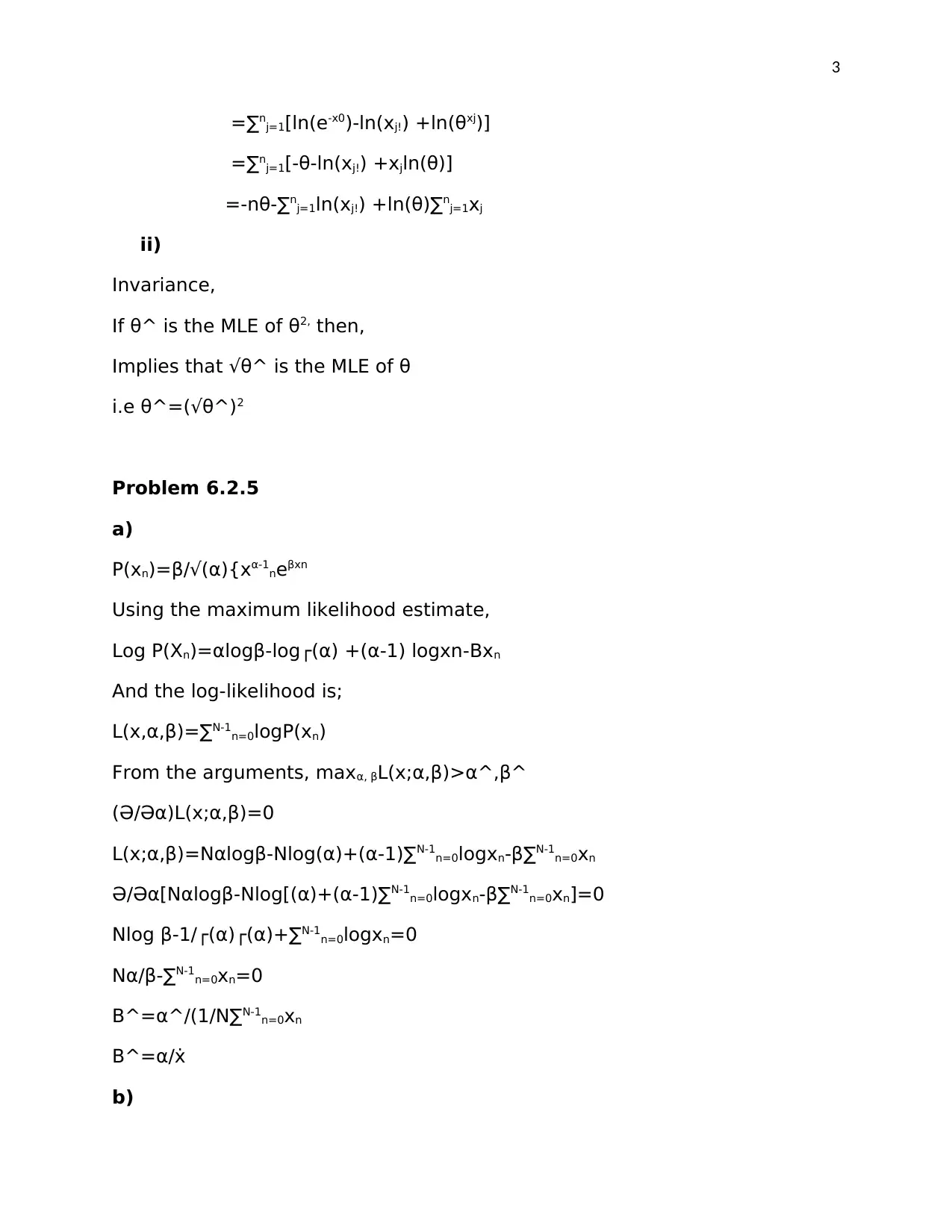
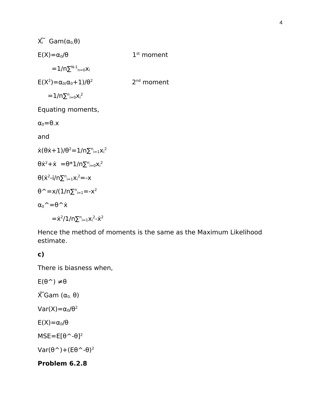
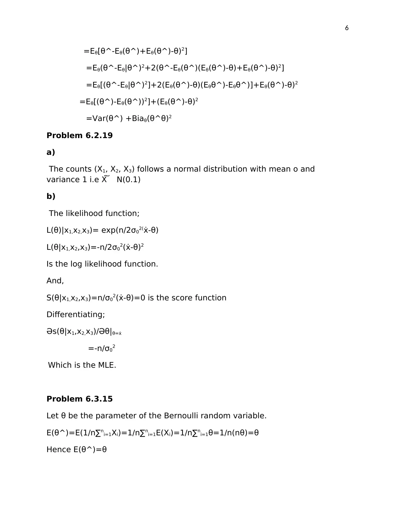
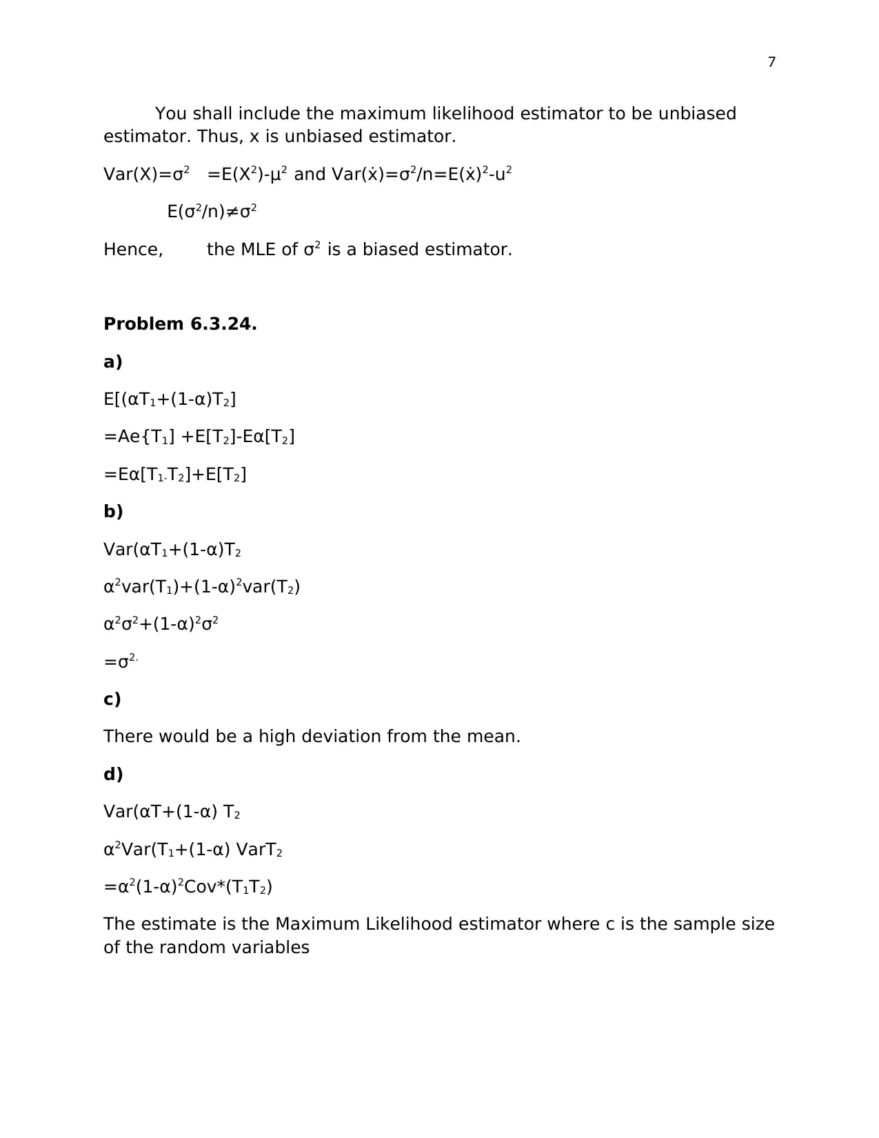
This document presents solutions to a set of probability and statistics problems, likely from a Statistics 630 course. The problems cover topics such as sufficient statistics, minimal sufficient statistics, maximum likelihood estimation (MLE), method of moments estimation, unbiased estimators, and properties of estimators like variance and bias. Specific problems address concepts related to Gamma distributions, Bernoulli random variables, and normal distributions. The solutions involve mathematical derivations, including likelihood functions, log-likelihood functions, score functions, and moment calculations. The document also references a paper on GMM estimators, suggesting a focus on advanced statistical methods. Desklib provides access to a wealth of student-contributed assignments and study resources to aid in understanding complex statistical concepts.

1
PROBABILITY & STATISTICS
Student’s Name:
University Affiliate:
Course:
Problem 6.1.7

2
L(X1,,…….,Xn)=(2pi σ2)-n/2exp(-1/2σ2)∑ni=1(xi-u)2)
=(2piσ2)-n/2exp(-n/2σ2(ẋ-u)2exp(-n-1/2σ2s2)
=Hence(ẋ,s2) is a sufficient statistic.
When μ is fixed at ẋ, we get,
L((ẋ,σ2)|x1,……,xn)=2 πσ2)-n/2exp(n-1/2σ2s2)
Maximized as a function of σ2
Therefore,
{ӘlnL((ẋ,σ2)|x)}/Әσ2=Ә/Әσ2(-n/2Inσ2-n-1/2σ2s2)
=-n/2σ2+(n-1/2σ4)s2
Problem 6.1.19
T(x) is a minimal sufficient statistic if and only if;
fθ(x)/fθ(x) is independent of θ ͢͢ T(x)=T(y) as a consequence of Fisher’s
factorization theorem.
Gamma fθ(x)=θα0/┌(α0)xα0-1eβx
fθ(Xn)/fθ(yn)=(∏ni=1θα0/┌(α0)xα0-1e-βxi)/(∏ni=1βα0/┌(α0)yα0-1e-βyi)
=(∏ni=1(xi)αo-1(∏ni=1yi)α0-1e∑xi/e∑yi
=(∏ni=1xi/∏ni=1yi)α-1e(∑yi-∑xi
=The minimum sufficient statistic for (α,θ)=(∏xi-∑ni=1xi
Problem 6.1.11
L(θ|X0)=θx0 =1
∫10L(θ|X0) =0
The likelihood is a constant, hence the integral of a constant is 0.
Problem 6.2.4
i) L(θ;x1,,……xn)=ln(∏nj=1exp(-θ2)1/xj!θ2xj
=- ∑nj=1ln(exp(-θ2)

3
=∑nj=1[ln(e-x0)-ln(xj!) +ln(θxj)]
=∑nj=1[-θ-ln(xj!) +xjln(θ)]
=-nθ-∑nj=1ln(xj!) +ln(θ)∑nj=1xj
ii)
Invariance,
If θ^ is the MLE of θ2, then,
Implies that √θ^ is the MLE of θ
i.e θ^=(√θ^)2
Problem 6.2.5
a)
P(xn)=β/√(α){xα-1neβxn
Using the maximum likelihood estimate,
Log P(Xn)=αlogβ-log┌(α) +(α-1) logxn-Bxn
And the log-likelihood is;
L(x,α,β)=∑N-1n=0logP(xn)
From the arguments, maxα, βL(x;α,β)>α^,β^
(Ә/Әα)L(x;α,β)=0
L(x;α,β)=Nαlogβ-Nlog(α)+(α-1)∑N-1n=0logxn-β∑N-1n=0xn
Ә/Әα[Nαlogβ-Nlog[(α)+(α-1)∑N-1n=0logxn-β∑N-1n=0xn]=0
Nlog β-1/┌(α)┌(α)+∑N-1n=0logxn=0
Nα/β-∑N-1n=0xn=0
Β^=α^/(1/N∑N-1n=0xn
Β^=α/ẋ
b)

4
Xi͠ Gam(α0,θ)
E(X)=α0/θ 1st moment
=1/n∑N-1n=0xi
E(X2)=α0(α0+1)/θ2 2nd moment
=1/n∑ni=0xi2
Equating moments,
α0=θ.x
and
ẋ(θẋ+1)/θ2=1/n∑ni=1xi2
θẋ2+ẋ =θ*1/n∑ni=0xi2
θ(ẋ2-i/n∑ni=1xi2=-x
θ^=x/(1/n∑ni=1=-x2
α0^=θ^ẋ
=ẋ2/1/n∑ni=1xi2-ẋ2
Hence the method of moments is the same as the Maximum Likelihood
estimate.
c)
There is biasness when,
E(θ^) ≠θ
X͠ Gam (α0, θ)
Var(X)=α0/θ2
E(X)=α0/θ
MSE=E[θ^-θ]2
Var(θ^)+(Eθ^-θ)2
Problem 6.2.8

5
L(X1,,……,Xn,θ)=∏fθ(xi)
Which when maximized gives;
L(X1,…..Xn,θ^)=supθ{∏ni=1fθ(xi)}
(Ә/Әθ)∏ni=1fθ(xi)=0
However, differentiating might be so cumbersome.
Alternatively;
When we maximize the log of likelihood, we get,
L(x1,…….xn,θ)=log(L(x1,,…..xn,θ)
=∑i=1nlog(fθ(xi)
L(x1,,……xn,θ^)=supθ{∑ni=0log(fθ(xi)}
Ә/Әθjl(x1,,,….Xn,θ^)=Ә/Әθj∑ni=1log(fθ(xi))
∑ni=0Ә/Әθjlog(fθ(xi)=0
Problem 6.2.12.
a)
L=F(x2,x2,…xn|θ)=f(x1|θ)*f(x2|θ)*………*f(xn|θ)
And the log –likelihood function is;
L^=1/nlogL=1/n∑ni=1logf(xi|θ)
The plug-in MLE of σ2 is identical to the likelihood function.
b)
E[s2]=E[1/n∑ni=0(Xi-μ)2-2/n(ẋ-μ)∑ni=1(xi-μ)+(ẋ)-μ)2]
=E(1/n∑ni=1(xi-μ)2-2/n(ẋ-μ).n.(ẋ-μ)+(ẋ-μ)2
=E[1/n∑ni=1(Xi-μ)2-(ẋ-μ)2
=E[1/n∑ni=0(xi-μ)-E[ẋ-μ)2]
=σ2-E[ẋ-μ)2]=(1-1/n)σ2<σ2
MSE(θ^)=Eθ[(θ^-θ)2]

6
=Eθ[θ^-Eθ(θ^)+Eθ(θ^)-θ)2]
=Eθ(θ^-Eθ|θ^)2+2(θ^-Eθ(θ^)(Eθ(θ^)-θ)+Eθ(θ^)-θ)2]
=Eθ[(θ^-Eθ|θ^)2]+2(Eθ(θ^)-θ)(Eθθ^)-Eθθ^)]+Eθ(θ^)-θ)2
=Eθ[(θ^)-Eθ(θ^))2]+(Eθ(θ^)-θ)2
=Var(θ^) +Biaθ(θ^θ)2
Problem 6.2.19
a)
The counts (X1, X2, X3) follows a normal distribution with mean o and
variance 1 i.e X͠ N(0.1)
b)
The likelihood function;
L(θ)|x1,x2,x3)= exp(n/2σ02(ẋ-θ)
L(θ|x1,x2,x3)=-n/2σ02(ẋ-θ)2
Is the log likelihood function.
And,
S(θ|x1,x2,x3)=n/σ02(ẋ-θ)=0 is the score function
Differentiating;
Әs(θ|x1,x2,x3)/Әθ|θ=ẋ
=-n/σ02
Which is the MLE.
Problem 6.3.15
Let θ be the parameter of the Bernoulli random variable.
E(θ^)=E(1/n∑ni=1Xi)=1/n∑ni=1E(Xi)=1/n∑ni=1θ=1/n(nθ)=θ
Hence E(θ^)=θ

7
You shall include the maximum likelihood estimator to be unbiased
estimator. Thus, x is unbiased estimator.
Var(X)=σ2 =E(X2)-μ2 and Var(ẋ)=σ2/n=E(ẋ)2-u2
E(σ2/n)≠σ2
Hence, the MLE of σ2 is a biased estimator.
Problem 6.3.24.
a)
E[(αT1+(1-α)T2]
=Αe{T1] +E[T2]-Eα[T2]
=Eα[T1-T2]+E[T2]
b)
Var(αT1+(1-α)T2
α2var(T1)+(1-α)2var(T2)
α2σ2+(1-α)2σ2
=σ2.
c)
There would be a high deviation from the mean.
d)
Var(αT+(1-α) T2
α2Var(T1+(1-α) VarT2
=α2(1-α)2Cov*(T1T2)
The estimate is the Maximum Likelihood estimator where c is the sample size
of the random variables

8
References:
Windmeijer, F., 2005. A finite sample correction for the variance of linear
efficient two-step GMM estimators. Journal of econometrics, 126(1), pp.25-
51.