Statistics Assignment 12: Statistical Analysis of Accident Death Data

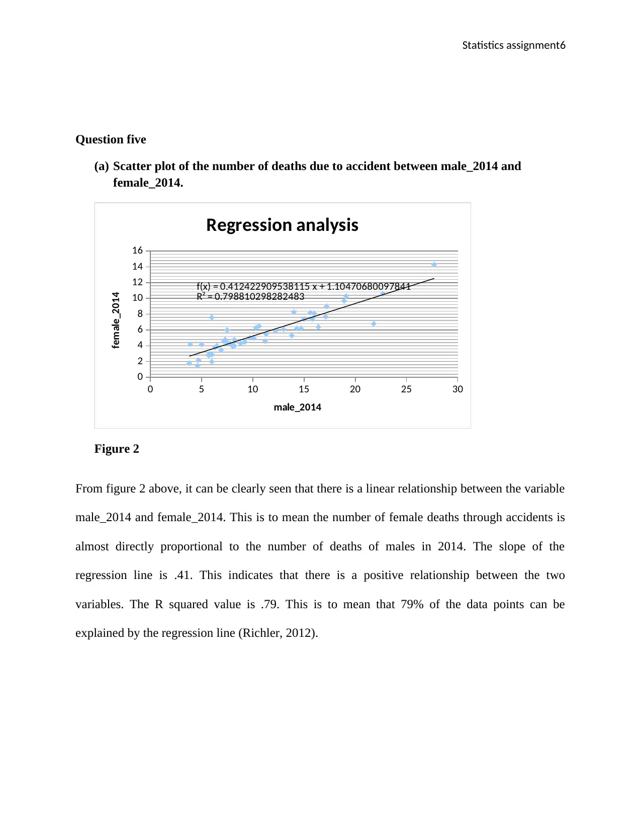
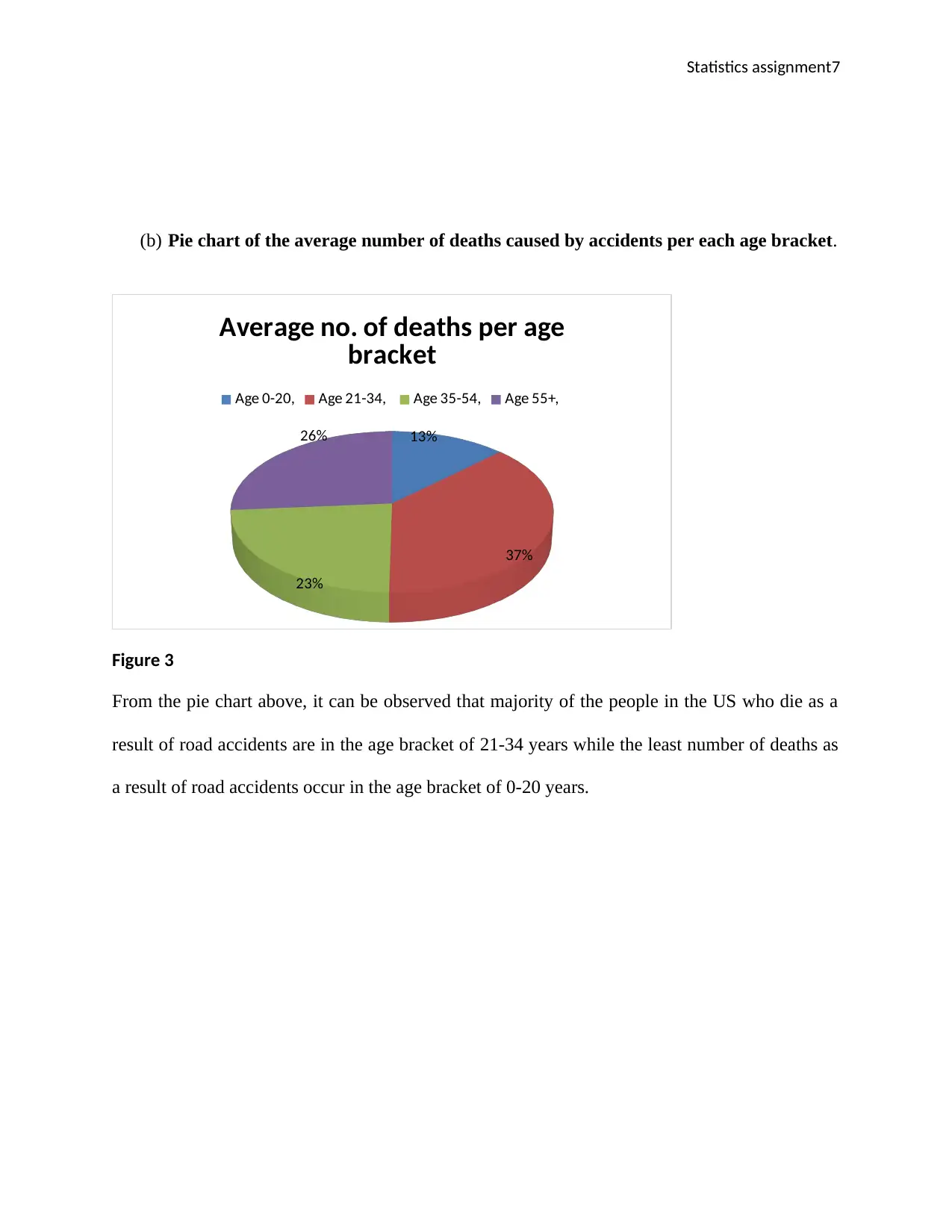
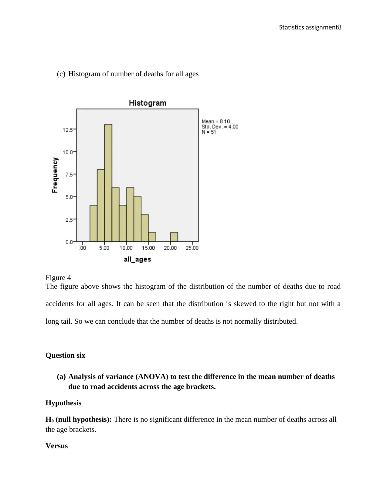
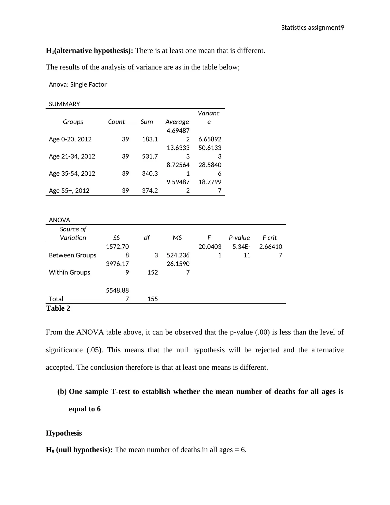
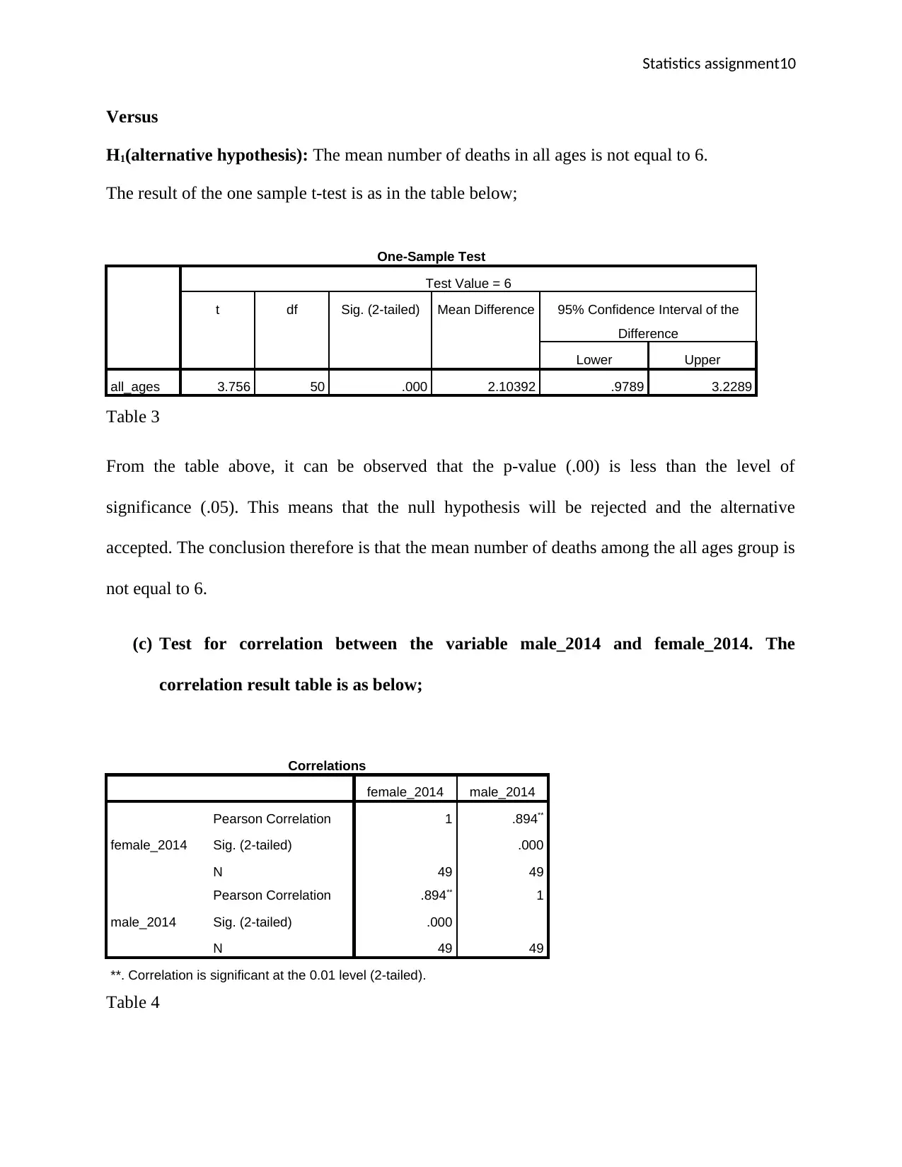
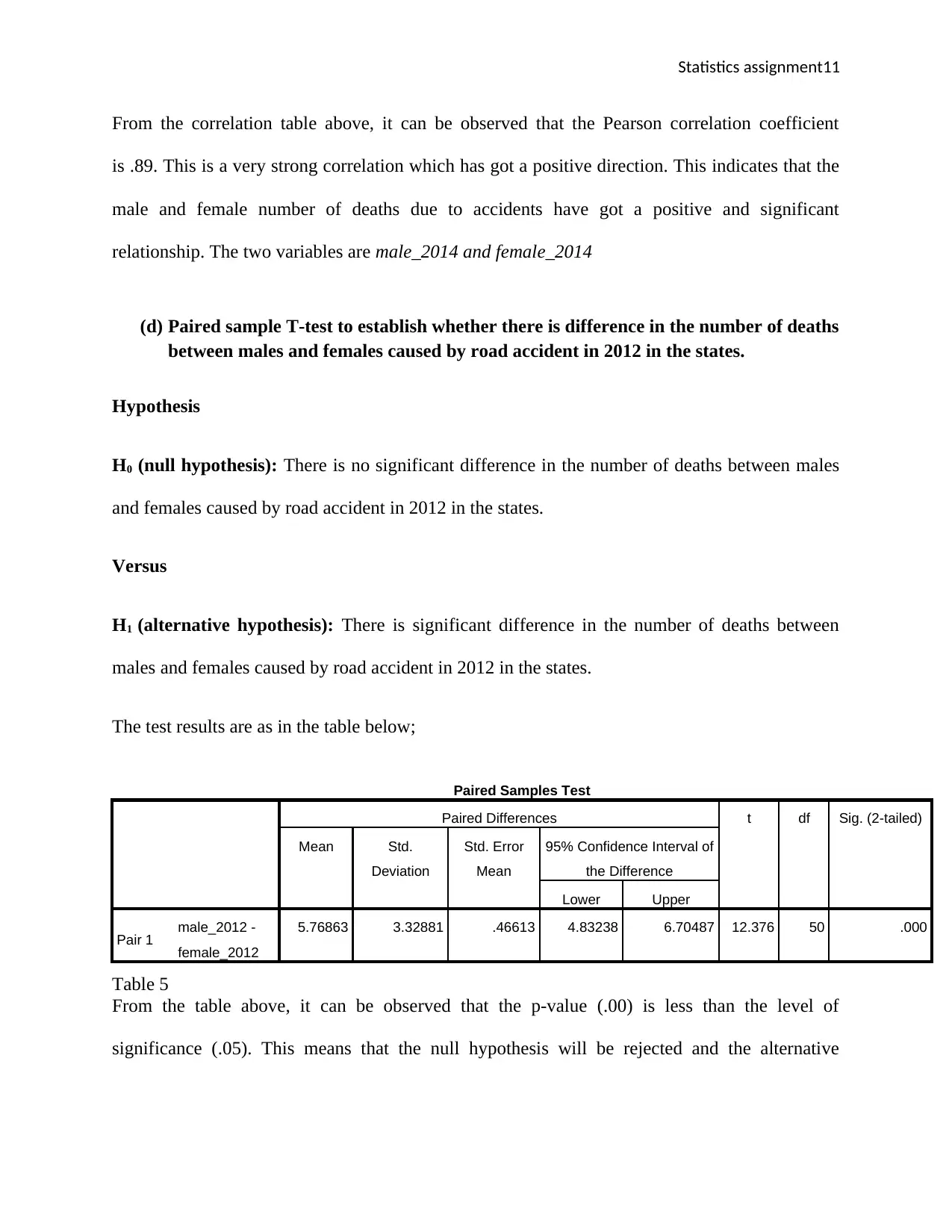
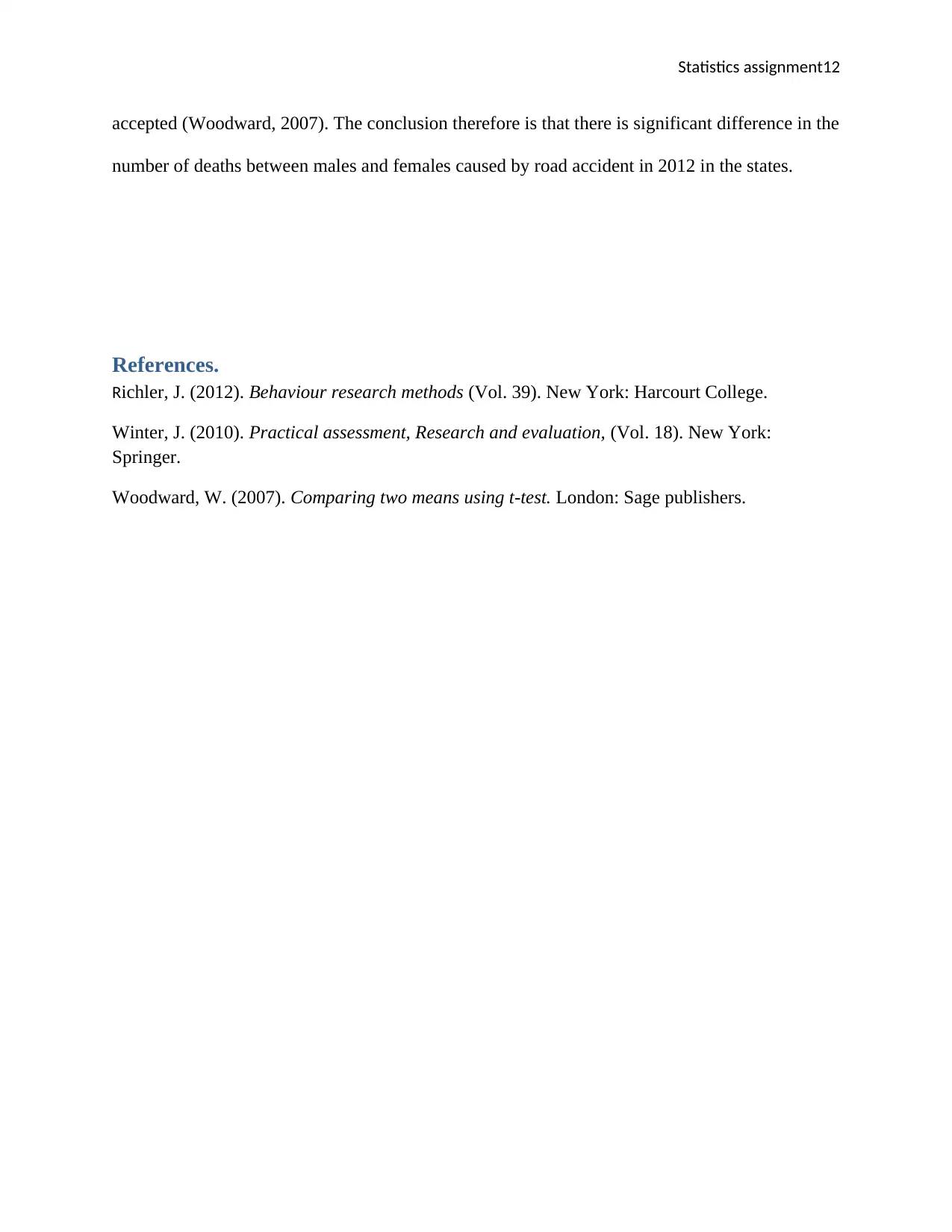
This statistics assignment analyzes accident death data across different states, considering age and gender. It explores dependent and independent variables, null and alternative hypotheses, and probability distributions. The assignment includes correlation tests between male and female deaths, regression analysis, and scatter plots. Furthermore, it utilizes ANOVA to compare the mean number of deaths across age brackets and a one-sample t-test to assess the mean number of deaths for all ages. Paired sample t-tests are also conducted to determine the difference in deaths between males and females. The analysis uses various statistical techniques to draw conclusions about accident-related deaths, providing insights into the data's characteristics and relationships between variables. The assignment also includes visual representations like histograms, scatter plots, and pie charts to aid in data interpretation. The results of the tests are interpreted and conclusions are drawn based on the statistical significance of the findings.

Statistics assignment1
Title
Student’s name
Professor
Course title
Date

Statistics assignment2
Question one
This data represents the number of deaths caused by accidents that have occurred in different
states and profiled according to age and gender. Therefore it this case a dependent or
independent variable can only be identified in the context of a given test. As they are now, any of
the variables can be a dependent or an independent variable according to how it is used in a
particular test. The data link is as provided below.
datalink
Question two
To explain a null hypothesis, let us use number of deaths of females in 2012 and the number of
deaths of males in the same year. We may want to establish whether there is a significant
difference in the number of females and males deaths that occur as a result of road accidents in
the various states. Ideally, since accident is not a planned event so that it just kills a particular
gender, we do not expect it to follow a particular pattern in claiming people of different genders.
So basing on this assumption, it is expected that the number of deaths due to accident among the
males should just be more or less the same number of deaths among the females that occur due to
accident. Therefore, a null hypothesis is always about maintaining a status quo (Winter, 2010);
how things are expected to be naturally. In this example, we can have the whole hypothesis about
the scenario as below;
Hypothesis
H0 (null hypothesis): There is no significant difference in the number of deaths between males
and females caused by road accident in 2012 in the states.

Statistics assignment3
Versus
H1(alternative hypothesis): There is no significant difference in the number of deaths between
males and females caused by road accident in 2012 in the states.
Question three
Probability distribution for the number of deaths for all ages
Figure 1
It can be observed from the histogram above that the number of deaths for all the ages in the
states is normally distributed. This is indicated by the normal distribution curve. The curve has a
sharp peak hence kurtic.

Statistics assignment4
Question four
(a) Test for correlation between number of deaths of males and females in 2012. The results
of the correlation test is as in the table below;
Correlations
male_2012 female_2012
male_2012
Pearson Correlation 1 .899**
Sig. (2-tailed) .000
N 51 51
female_2012
Pearson Correlation .899** 1
Sig. (2-tailed) .000
N 51 51
**. Correlation is significant at the 0.01 level (2-tailed).
Table 1
From the correlation table above, it can be observed that the Pearson correlation coefficient
is .89. This is a very strong correlation which has got a positive direction. This indicates that the
male and female number of deaths due to accidents have got a positive and significant
relationship. The two variables are male_2012 and female_2012

Statistics assignment5
(b) Regression line between the variables male_2012 and female_2012
0 5 10 15 20 25 30 35
0
2
4
6
8
10
12
14
f(x) = 0.453271497967188 x + 0.418069375320419
R² = 0.810448471655048
Regression analysis
male_2012
female_2012
Figure 1
From figure 1 above, it can be clearly seen that there is a linear relationship between the variable
male_2012 and female_2012. This is to mean the number of female deaths through accidents is
almost directly proportional to the number of deaths of males in 2012. The slope of the
regression line is .45. This indicates that there is a positive relationship between the two
variables. The R squared value is .81. This is to mean that 81% of the data points can be
explained by the regression line.

Statistics assignment6
Question five
(a) Scatter plot of the number of deaths due to accident between male_2014 and
female_2014.
0 5 10 15 20 25 30
0
2
4
6
8
10
12
14
16
f(x) = 0.412422909538115 x + 1.10470680097841
R² = 0.798810298282483
Regression analysis
male_2014
female_2014
Figure 2
From figure 2 above, it can be clearly seen that there is a linear relationship between the variable
male_2014 and female_2014. This is to mean the number of female deaths through accidents is
almost directly proportional to the number of deaths of males in 2014. The slope of the
regression line is .41. This indicates that there is a positive relationship between the two
variables. The R squared value is .79. This is to mean that 79% of the data points can be
explained by the regression line (Richler, 2012).

Statistics assignment7
(b) Pie chart of the average number of deaths caused by accidents per each age bracket.
13%
37%
23%
26%
Average no. of deaths per age
bracket
Age 0-20, Age 21-34, Age 35-54, Age 55+,
Figure 3
From the pie chart above, it can be observed that majority of the people in the US who die as a
result of road accidents are in the age bracket of 21-34 years while the least number of deaths as
a result of road accidents occur in the age bracket of 0-20 years.

Statistics assignment8
(c) Histogram of number of deaths for all ages
Figure 4
The figure above shows the histogram of the distribution of the number of deaths due to road
accidents for all ages. It can be seen that the distribution is skewed to the right but not with a
long tail. So we can conclude that the number of deaths is not normally distributed.
Question six
(a) Analysis of variance (ANOVA) to test the difference in the mean number of deaths
due to road accidents across the age brackets.
Hypothesis
H0 (null hypothesis): There is no significant difference in the mean number of deaths across all
the age brackets.
Versus

Statistics assignment9
H1(alternative hypothesis): There is at least one mean that is different.
The results of the analysis of variance are as in the table below;
Anova: Single Factor
SUMMARY
Groups Count Sum Average
Varianc
e
Age 0-20, 2012 39 183.1
4.69487
2 6.65892
Age 21-34, 2012 39 531.7
13.6333
3
50.6133
3
Age 35-54, 2012 39 340.3
8.72564
1
28.5840
6
Age 55+, 2012 39 374.2
9.59487
2
18.7799
7
ANOVA
Source of
Variation SS df MS F P-value F crit
Between Groups
1572.70
8 3 524.236
20.0403
1
5.34E-
11
2.66410
7
Within Groups
3976.17
9 152
26.1590
7
Total
5548.88
7 155
Table 2
From the ANOVA table above, it can be observed that the p-value (.00) is less than the level of
significance (.05). This means that the null hypothesis will be rejected and the alternative
accepted. The conclusion therefore is that at least one means is different.
(b) One sample T-test to establish whether the mean number of deaths for all ages is
equal to 6
Hypothesis
H0 (null hypothesis): The mean number of deaths in all ages = 6.

Statistics assignment10
Versus
H1(alternative hypothesis): The mean number of deaths in all ages is not equal to 6.
The result of the one sample t-test is as in the table below;
One-Sample Test
Test Value = 6
t df Sig. (2-tailed) Mean Difference 95% Confidence Interval of the
Difference
Lower Upper
all_ages 3.756 50 .000 2.10392 .9789 3.2289
Table 3
From the table above, it can be observed that the p-value (.00) is less than the level of
significance (.05). This means that the null hypothesis will be rejected and the alternative
accepted. The conclusion therefore is that the mean number of deaths among the all ages group is
not equal to 6.
(c) Test for correlation between the variable male_2014 and female_2014. The
correlation result table is as below;
Correlations
female_2014 male_2014
female_2014
Pearson Correlation 1 .894**
Sig. (2-tailed) .000
N 49 49
male_2014
Pearson Correlation .894** 1
Sig. (2-tailed) .000
N 49 49
**. Correlation is significant at the 0.01 level (2-tailed).
Table 4

Statistics assignment11
From the correlation table above, it can be observed that the Pearson correlation coefficient
is .89. This is a very strong correlation which has got a positive direction. This indicates that the
male and female number of deaths due to accidents have got a positive and significant
relationship. The two variables are male_2014 and female_2014
(d) Paired sample T-test to establish whether there is difference in the number of deaths
between males and females caused by road accident in 2012 in the states.
Hypothesis
H0 (null hypothesis): There is no significant difference in the number of deaths between males
and females caused by road accident in 2012 in the states.
Versus
H1 (alternative hypothesis): There is significant difference in the number of deaths between
males and females caused by road accident in 2012 in the states.
The test results are as in the table below;
Paired Samples Test
Paired Differences t df Sig. (2-tailed)
Mean Std.
Deviation
Std. Error
Mean
95% Confidence Interval of
the Difference
Lower Upper
Pair 1 male_2012 -
female_2012
5.76863 3.32881 .46613 4.83238 6.70487 12.376 50 .000
Table 5
From the table above, it can be observed that the p-value (.00) is less than the level of
significance (.05). This means that the null hypothesis will be rejected and the alternative

Statistics assignment12
accepted (Woodward, 2007). The conclusion therefore is that there is significant difference in the
number of deaths between males and females caused by road accident in 2012 in the states.
References.
Richler, J. (2012). Behaviour research methods (Vol. 39). New York: Harcourt College.
Winter, J. (2010). Practical assessment, Research and evaluation, (Vol. 18). New York:
Springer.
Woodward, W. (2007). Comparing two means using t-test. London: Sage publishers.