Statistics for Management: Income, Earnings, and Regression Analysis
VerifiedAdded on 2020/06/06
|20
|3454
|98
Report
AI Summary
This report presents a comprehensive statistical analysis of various business-related data. It begins by examining income trends in the public and private sectors, including changes in gross annual income and the gap between male and female earnings. The report then delves into hourly earnings data, calculating descriptive statistics like mean and standard deviation, and constructing an Ogive chart to analyze the distribution of earnings. Further analysis includes the relationship between floor area and weekly turnover, calculating the correlation coefficient and evaluating the statistical validity of the model. The report also explores the economic order quantity (EOQ) and its implications for delivery management. Finally, the report concludes with scatter diagrams, income level comparisons across genders and sectors, and male gross annual earnings in the public sector, providing a holistic view of the data and its implications for management decisions.
STATISTICS FOR MANAGEMENT
Paraphrase This Document
Need a fresh take? Get an instant paraphrase of this document with our AI Paraphraser
TABLE OF CONTENTS
INTRODUCTION.......................................................................................................................................3
TASK 1.......................................................................................................................................................3
1Introduction of change in gross annual income across private and public sector...................................3
2 Gap between male and female income.................................................................................................5
TASK 2.......................................................................................................................................................5
(A)Analysis of hourly earnings data........................................................................................................5
(2) Calculation of descriptive statistics....................................................................................................6
(b)Comparison of results.........................................................................................................................8
(A)Floor area and weekly turnover..........................................................................................................8
© Calculation of turnover when value of size given..............................................................................11
(d) Calculation of correlation coefficient...............................................................................................12
(e) Statistical validity of model..............................................................................................................12
TASK 3.....................................................................................................................................................13
(a)Number of delivery made on annual basis.........................................................................................13
(b) Deliveries made on each round........................................................................................................13
©Economic order quantity.....................................................................................................................14
(d) Comparison of EOQ and cost...........................................................................................................14
TASK 4.....................................................................................................................................................15
(a)Scatter diagram of size and turnover.................................................................................................15
(b) Income level of gender in public and private sector.........................................................................17
(c)Male gross annual earning for public................................................................................................18
CONCLUSION.........................................................................................................................................19
...............................................................................................................................................................19
REFERENCES..........................................................................................................................................20
Figure 4Public and private sector male income level...................................................................................5
Figure 5Public and private sector female income level...............................................................................5
Figure6 Ogive chart.....................................................................................................................................7
Figure8 Relationship between size and turnover.........................................................................................9
Figure 9Turnover chart..............................................................................................................................17
Figure10 Trend in gross income across gender and public as well as private sector..................................18
Table 1Change in public and private sector income....................................................................................4
Table 2Gap between male and female income............................................................................................6
Table 2Data for Ogive.................................................................................................................................6
Table 3Calculation of mean.........................................................................................................................7
Table 4Input for computing standard deviation...........................................................................................8
Table 6Number of bottles transported.......................................................................................................14
Table7 Calculation of economic order quantity.........................................................................................15
Table 8 Cost at different level of EOQ......................................................................................................15
⊘ This is a preview!⊘
Do you want full access?
Subscribe today to unlock all pages.
Trusted by 1+ million students worldwide
INTRODUCTION
Statistics is one of the most important area that is proving very helpful to managers for making
business decisions. In current report income related trends are analyzed in respect to public and private
sector and charting of same is done to identify trends that remain in existence. Regression analysis
technique is also applied on dataset in order to identify relationship that exists between dependent and
independent variables. On the basis of correlation coefficient relationship between variables is find out
validity of model is evaluated. In this way it is determined that reliable results are obtained from model.
TASK 1
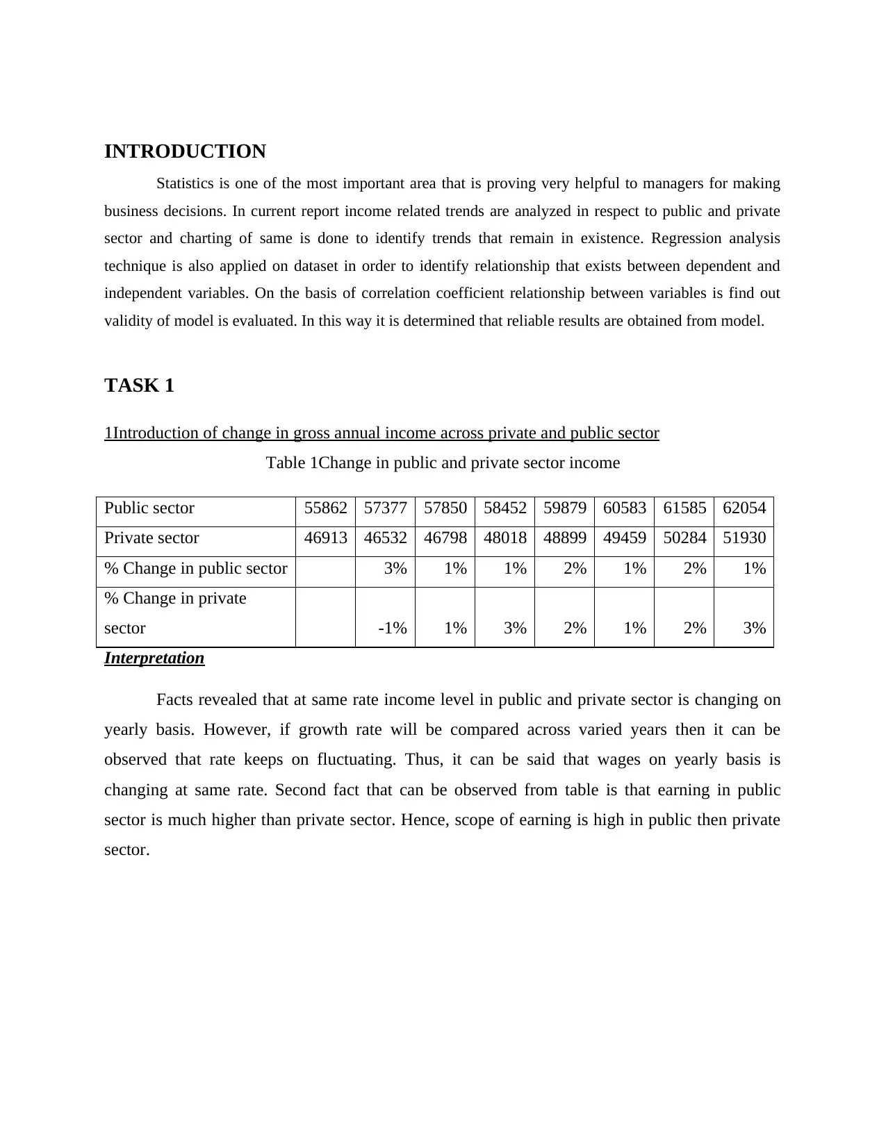
1Introduction of change in gross annual income across private and public sector
Table 1Change in public and private sector income
Public sector 55862 57377 57850 58452 59879 60583 61585 62054
Private sector 46913 46532 46798 48018 48899 49459 50284 51930
% Change in public sector 3% 1% 1% 2% 1% 2% 1%
% Change in private
sector -1% 1% 3% 2% 1% 2% 3%
Interpretation
Facts revealed that at same rate income level in public and private sector is changing on
yearly basis. However, if growth rate will be compared across varied years then it can be
observed that rate keeps on fluctuating. Thus, it can be said that wages on yearly basis is
changing at same rate. Second fact that can be observed from table is that earning in public
sector is much higher than private sector. Hence, scope of earning is high in public then private
sector.
Statistics is one of the most important area that is proving very helpful to managers for making
business decisions. In current report income related trends are analyzed in respect to public and private
sector and charting of same is done to identify trends that remain in existence. Regression analysis
technique is also applied on dataset in order to identify relationship that exists between dependent and
independent variables. On the basis of correlation coefficient relationship between variables is find out
validity of model is evaluated. In this way it is determined that reliable results are obtained from model.
TASK 1
1Introduction of change in gross annual income across private and public sector
Table 1Change in public and private sector income
Public sector 55862 57377 57850 58452 59879 60583 61585 62054
Private sector 46913 46532 46798 48018 48899 49459 50284 51930
% Change in public sector 3% 1% 1% 2% 1% 2% 1%
% Change in private
sector -1% 1% 3% 2% 1% 2% 3%
Interpretation
Facts revealed that at same rate income level in public and private sector is changing on
yearly basis. However, if growth rate will be compared across varied years then it can be
observed that rate keeps on fluctuating. Thus, it can be said that wages on yearly basis is
changing at same rate. Second fact that can be observed from table is that earning in public
sector is much higher than private sector. Hence, scope of earning is high in public then private
sector.
Paraphrase This Document
Need a fresh take? Get an instant paraphrase of this document with our AI Paraphraser
2009 2010 2011 2012 2013 2014 2015 2016
0
5000
10000
15000
20000
25000
30000
35000
40000
30638 31264313803181632541 328783368534011
27362 27000272332770528201 284422888129679
Public sector male
Private sector male
Figure 1Public and private sector male income level
2009 2010 2011 2012 2013 2014 2015 2016
0
10000
20000
30000
40000
50000
60000
70000
2522426113264702663627338277052790028053
19551195321956520313206982101721403
63690
Public sector female
Private sector female
Figure 2Public and private sector female income level
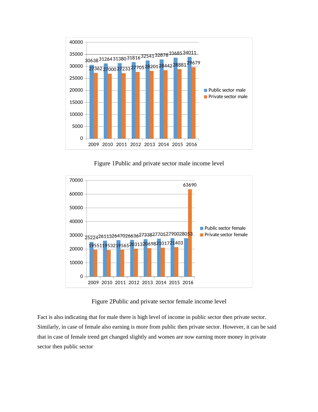
Fact is also indicating that for male there is high level of income in public sector then private sector.
Similarly, in case of female also earning is more from public then private sector. However, it can be said
that in case of female trend get changed slightly and women are now earning more money in private
sector then public sector
0
5000
10000
15000
20000
25000
30000
35000
40000
30638 31264313803181632541 328783368534011
27362 27000272332770528201 284422888129679
Public sector male
Private sector male
Figure 1Public and private sector male income level
2009 2010 2011 2012 2013 2014 2015 2016
0
10000
20000
30000
40000
50000
60000
70000
2522426113264702663627338277052790028053
19551195321956520313206982101721403
63690
Public sector female
Private sector female
Figure 2Public and private sector female income level
Fact is also indicating that for male there is high level of income in public sector then private sector.
Similarly, in case of female also earning is more from public then private sector. However, it can be said
that in case of female trend get changed slightly and women are now earning more money in private
sector then public sector
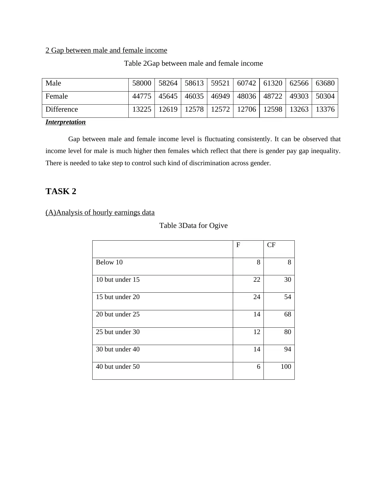
2 Gap between male and female income
Table 2Gap between male and female income
Male 58000 58264 58613 59521 60742 61320 62566 63680
Female 44775 45645 46035 46949 48036 48722 49303 50304
Difference 13225 12619 12578 12572 12706 12598 13263 13376
Interpretation
Gap between male and female income level is fluctuating consistently. It can be observed that
income level for male is much higher then females which reflect that there is gender pay gap inequality.
There is needed to take step to control such kind of discrimination across gender.
TASK 2
(A)Analysis of hourly earnings data
Table 3Data for Ogive
F CF
Below 10 8 8
10 but under 15 22 30
15 but under 20 24 54
20 but under 25 14 68
25 but under 30 12 80
30 but under 40 14 94
40 but under 50 6 100
⊘ This is a preview!⊘
Do you want full access?
Subscribe today to unlock all pages.
Trusted by 1+ million students worldwide
Below 10 10 but under
15 15 but under
20 20 but under
25 25 but under
30 30 but under
40 40 but under
50
0
20
40
60
80
100
120
8
30
54
68
80
94 100
Chart Title
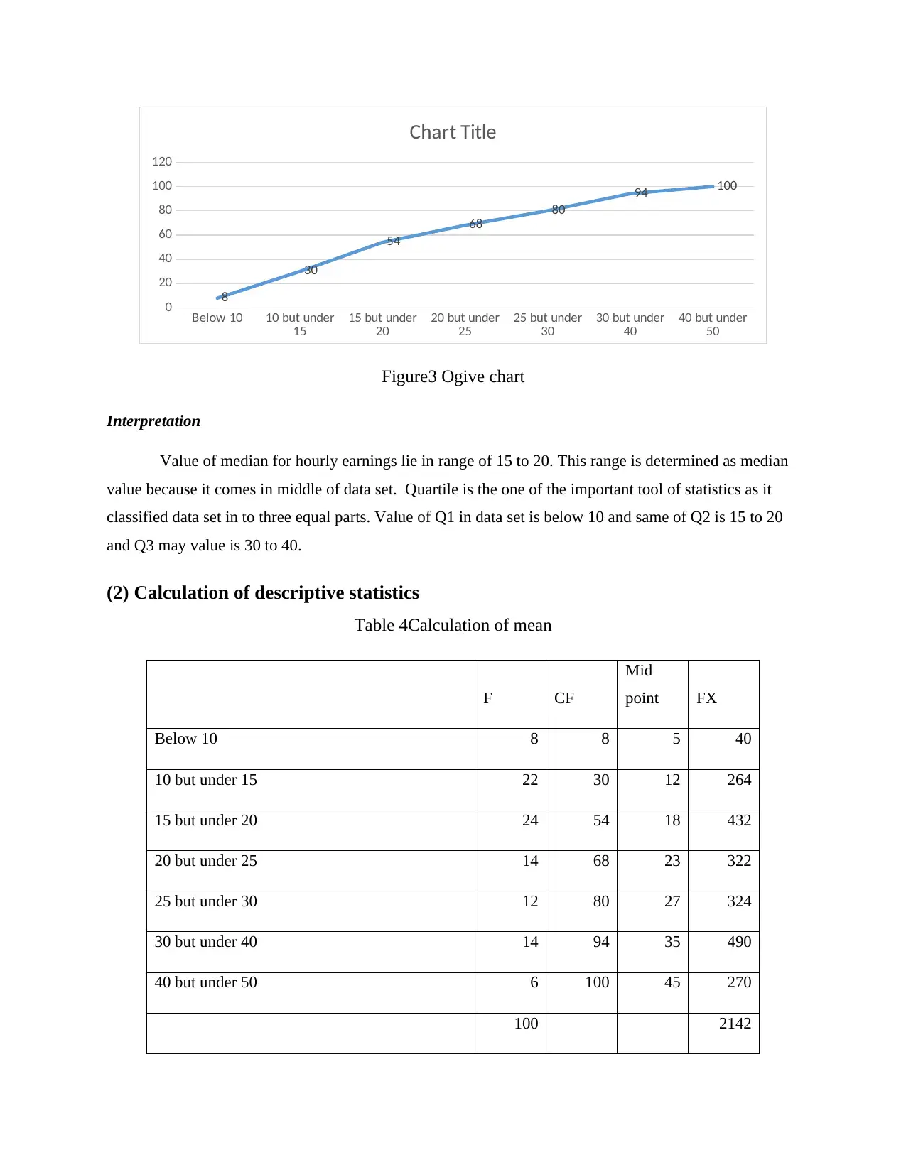
Figure3 Ogive chart
Interpretation
Value of median for hourly earnings lie in range of 15 to 20. This range is determined as median
value because it comes in middle of data set. Quartile is the one of the important tool of statistics as it
classified data set in to three equal parts. Value of Q1 in data set is below 10 and same of Q2 is 15 to 20
and Q3 may value is 30 to 40.
(2) Calculation of descriptive statistics
Table 4Calculation of mean
F CF
Mid
point FX
Below 10 8 8 5 40
10 but under 15 22 30 12 264
15 but under 20 24 54 18 432
20 but under 25 14 68 23 322
25 but under 30 12 80 27 324
30 but under 40 14 94 35 490
40 but under 50 6 100 45 270
100 2142
15 15 but under
20 20 but under
25 25 but under
30 30 but under
40 40 but under
50
0
20
40
60
80
100
120
8
30
54
68
80
94 100
Chart Title
Figure3 Ogive chart
Interpretation
Value of median for hourly earnings lie in range of 15 to 20. This range is determined as median
value because it comes in middle of data set. Quartile is the one of the important tool of statistics as it
classified data set in to three equal parts. Value of Q1 in data set is below 10 and same of Q2 is 15 to 20
and Q3 may value is 30 to 40.
(2) Calculation of descriptive statistics
Table 4Calculation of mean
F CF
Mid
point FX
Below 10 8 8 5 40
10 but under 15 22 30 12 264
15 but under 20 24 54 18 432
20 but under 25 14 68 23 322
25 but under 30 12 80 27 324
30 but under 40 14 94 35 490
40 but under 50 6 100 45 270
100 2142
Paraphrase This Document
Need a fresh take? Get an instant paraphrase of this document with our AI Paraphraser
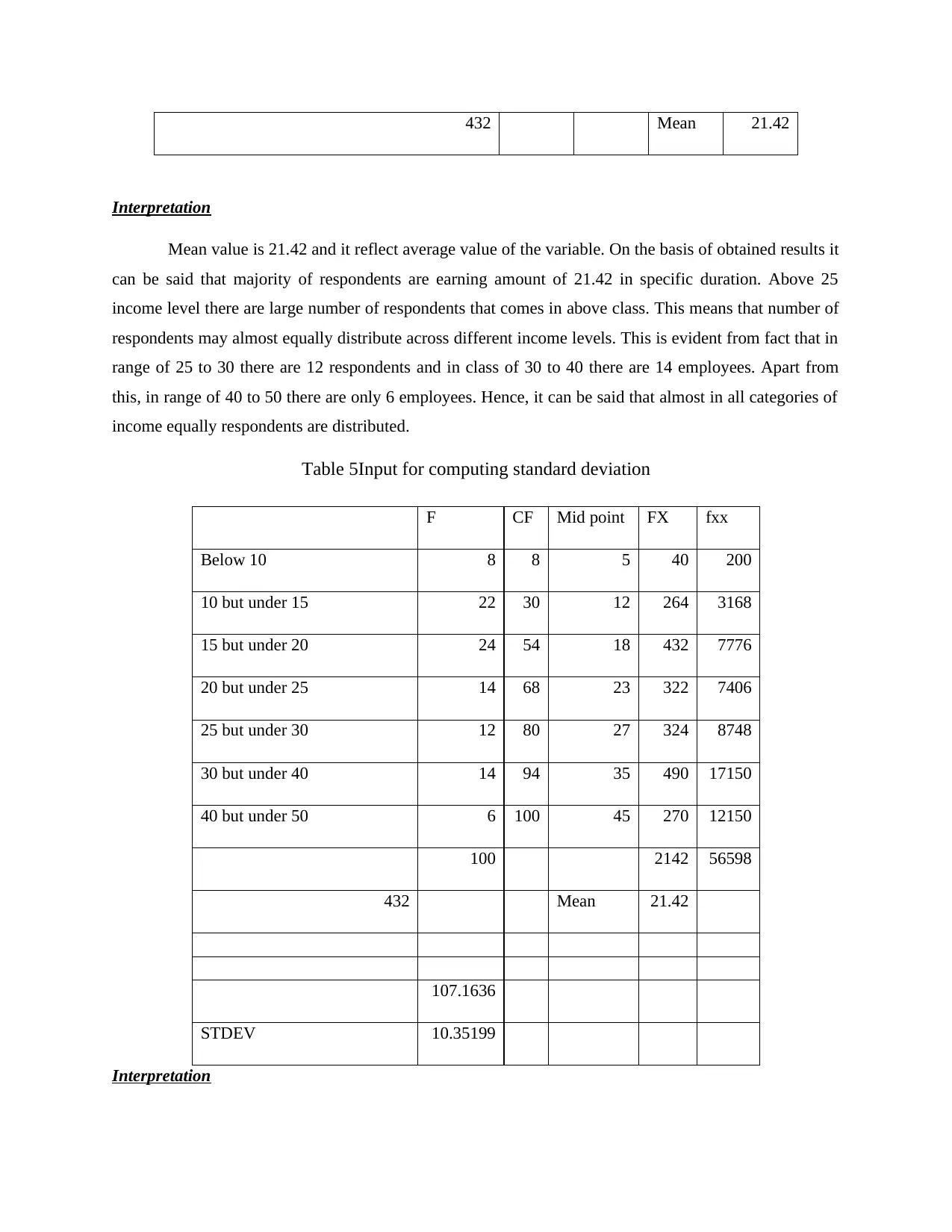
432 Mean 21.42
Interpretation
Mean value is 21.42 and it reflect average value of the variable. On the basis of obtained results it
can be said that majority of respondents are earning amount of 21.42 in specific duration. Above 25
income level there are large number of respondents that comes in above class. This means that number of
respondents may almost equally distribute across different income levels. This is evident from fact that in
range of 25 to 30 there are 12 respondents and in class of 30 to 40 there are 14 employees. Apart from
this, in range of 40 to 50 there are only 6 employees. Hence, it can be said that almost in all categories of
income equally respondents are distributed.
Table 5Input for computing standard deviation
F CF Mid point FX fxx
Below 10 8 8 5 40 200
10 but under 15 22 30 12 264 3168
15 but under 20 24 54 18 432 7776
20 but under 25 14 68 23 322 7406
25 but under 30 12 80 27 324 8748
30 but under 40 14 94 35 490 17150
40 but under 50 6 100 45 270 12150
100 2142 56598
432 Mean 21.42
107.1636
STDEV 10.35199
Interpretation
Interpretation
Mean value is 21.42 and it reflect average value of the variable. On the basis of obtained results it
can be said that majority of respondents are earning amount of 21.42 in specific duration. Above 25
income level there are large number of respondents that comes in above class. This means that number of
respondents may almost equally distribute across different income levels. This is evident from fact that in
range of 25 to 30 there are 12 respondents and in class of 30 to 40 there are 14 employees. Apart from
this, in range of 40 to 50 there are only 6 employees. Hence, it can be said that almost in all categories of
income equally respondents are distributed.
Table 5Input for computing standard deviation
F CF Mid point FX fxx
Below 10 8 8 5 40 200
10 but under 15 22 30 12 264 3168
15 but under 20 24 54 18 432 7776
20 but under 25 14 68 23 322 7406
25 but under 30 12 80 27 324 8748
30 but under 40 14 94 35 490 17150
40 but under 50 6 100 45 270 12150
100 2142 56598
432 Mean 21.42
107.1636
STDEV 10.35199
Interpretation
Standard deviation is the one of the most important tool because it reflects extent to which values
of variable are deviating from their mean value (Descriptive and inferential statistics, 2017). It can be
observed that value of standard deviation is only 10.35 which mean that values are deviating at very slow
rate and due to this reason there is less variance in data set. It can be said that salary of employees is
deviating at very slow rate.
(b)Comparison of results
Results on comparison are indicating that in case of South portion of England there is higher
amount of annual earning then North portion of England. It can also be seen that values are deviating at
very slow rate 7.40 in case of Noth eastern part which is very low and along with this salary is high. This
means that in case of South Eastern part heavy amount is earned then North Eastern area of England.
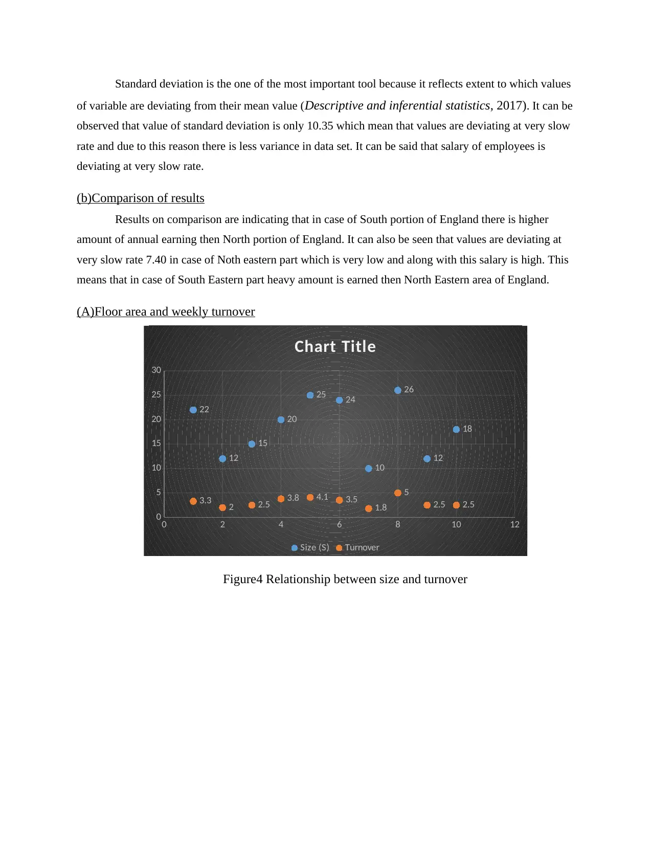
(A)Floor area and weekly turnover
0 2 4 6 8 10 12
0
5
10
15
20
25
30
3.3 2 2.5 3.8 4.1 3.5 1.8
5
2.5 2.5
22
12
15
20
25 24
10
26
12
18
Chart Title
Size (S) Turnover
Figure4 Relationship between size and turnover
of variable are deviating from their mean value (Descriptive and inferential statistics, 2017). It can be
observed that value of standard deviation is only 10.35 which mean that values are deviating at very slow
rate and due to this reason there is less variance in data set. It can be said that salary of employees is
deviating at very slow rate.
(b)Comparison of results
Results on comparison are indicating that in case of South portion of England there is higher
amount of annual earning then North portion of England. It can also be seen that values are deviating at
very slow rate 7.40 in case of Noth eastern part which is very low and along with this salary is high. This
means that in case of South Eastern part heavy amount is earned then North Eastern area of England.
(A)Floor area and weekly turnover
0 2 4 6 8 10 12
0
5
10
15
20
25
30
3.3 2 2.5 3.8 4.1 3.5 1.8
5
2.5 2.5
22
12
15
20
25 24
10
26
12
18
Chart Title
Size (S) Turnover
Figure4 Relationship between size and turnover
⊘ This is a preview!⊘
Do you want full access?
Subscribe today to unlock all pages.
Trusted by 1+ million students worldwide
0 2 4 6 8 10 12
0
2
4
6
8
10
12
f(x) = NaN x + NaN
R² = 0 Size (S)
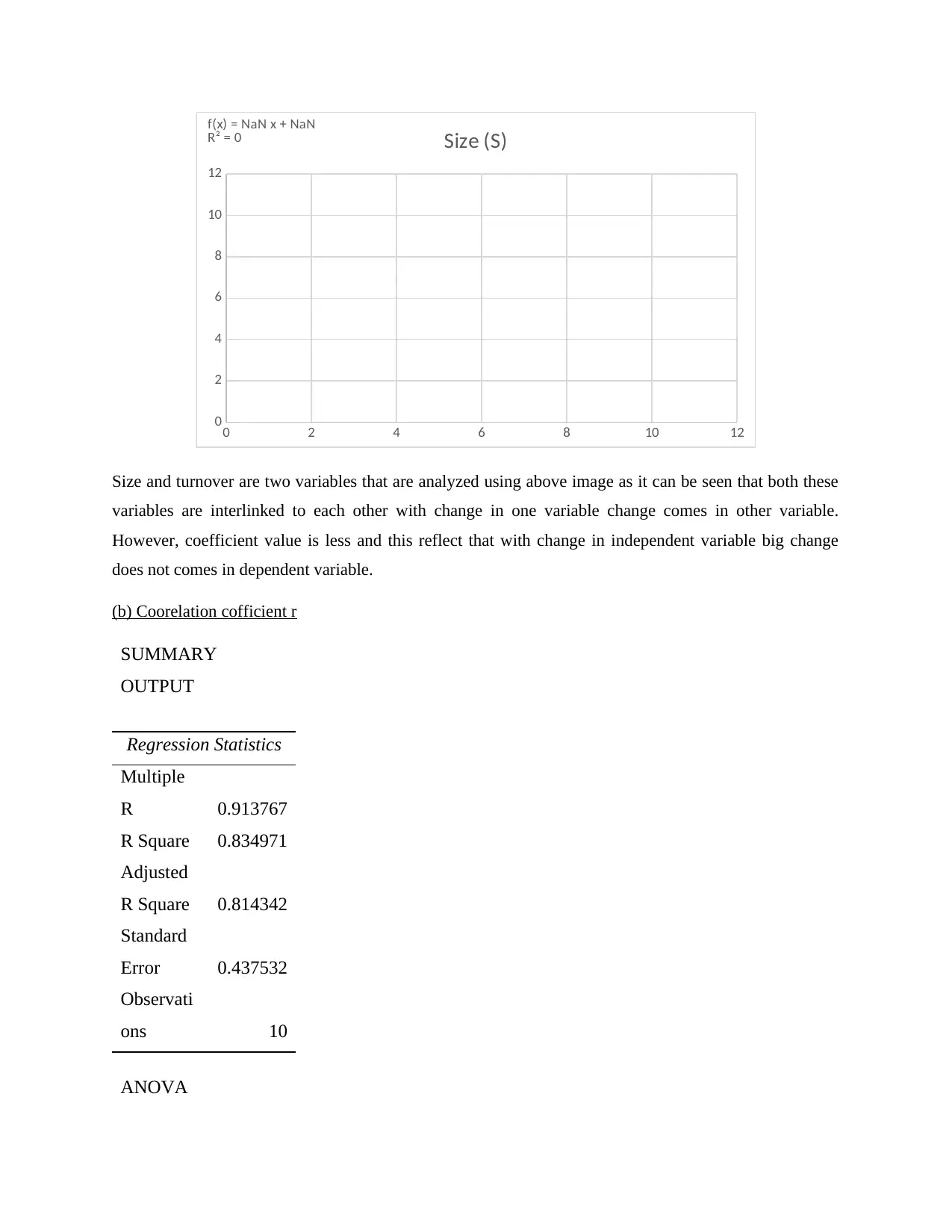
Size and turnover are two variables that are analyzed using above image as it can be seen that both these
variables are interlinked to each other with change in one variable change comes in other variable.
However, coefficient value is less and this reflect that with change in independent variable big change
does not comes in dependent variable.
(b) Coorelation cofficient r
SUMMARY
OUTPUT
Regression Statistics
Multiple
R 0.913767
R Square 0.834971
Adjusted
R Square 0.814342
Standard
Error 0.437532
Observati
ons 10
ANOVA
0
2
4
6
8
10
12
f(x) = NaN x + NaN
R² = 0 Size (S)
Size and turnover are two variables that are analyzed using above image as it can be seen that both these
variables are interlinked to each other with change in one variable change comes in other variable.
However, coefficient value is less and this reflect that with change in independent variable big change
does not comes in dependent variable.
(b) Coorelation cofficient r
SUMMARY
OUTPUT
Regression Statistics
Multiple
R 0.913767
R Square 0.834971
Adjusted
R Square 0.814342
Standard
Error 0.437532
Observati
ons 10
ANOVA
Paraphrase This Document
Need a fresh take? Get an instant paraphrase of this document with our AI Paraphraser
df SS MS F
Significa
nce F
Regressio
n 1
7.7485
28 7.748528
40.476
22 0.000218
Residual 8
1.5314
72 0.191434
Total 9 9.28
Coefficie
nts
Standa
rd
Error t Stat
P-
value
Lower
95%
Upper
95%
Lower
95.0%
Upper
95.0%
Intercept 0.202177
0.4760
34 0.424711
0.6822
39 -0.89556
1.2999
12
-
0.8955
6
1.2999
12
Size (S) 0.15749
0.0247
54 6.362093
0.0002
18 0.100406
0.2145
74
0.1004
06
0.2145
74
RESIDUAL
OUTPUT
Observati
on
Predicte
d
Turnover
Residu
als
Standard
Residual
s
1 3.666965
-
0.3669
7 -0.88959
2 2.092061
-
0.0920
6 -0.22317
3 2.564533 -
0.0645
-0.15644
3
4 3.351985
0.4480
15 1.086074
5 4.139437
-
0.0394
4 -0.0956
6 3.981946
-
0.4819
5 -1.16833
7 1.777081
0.0229
19 0.055561
8 4.296927
0.7030
73 1.704383
9 2.092061
0.4079
39 0.988921
10 3.037004 -0.537 -1.3018
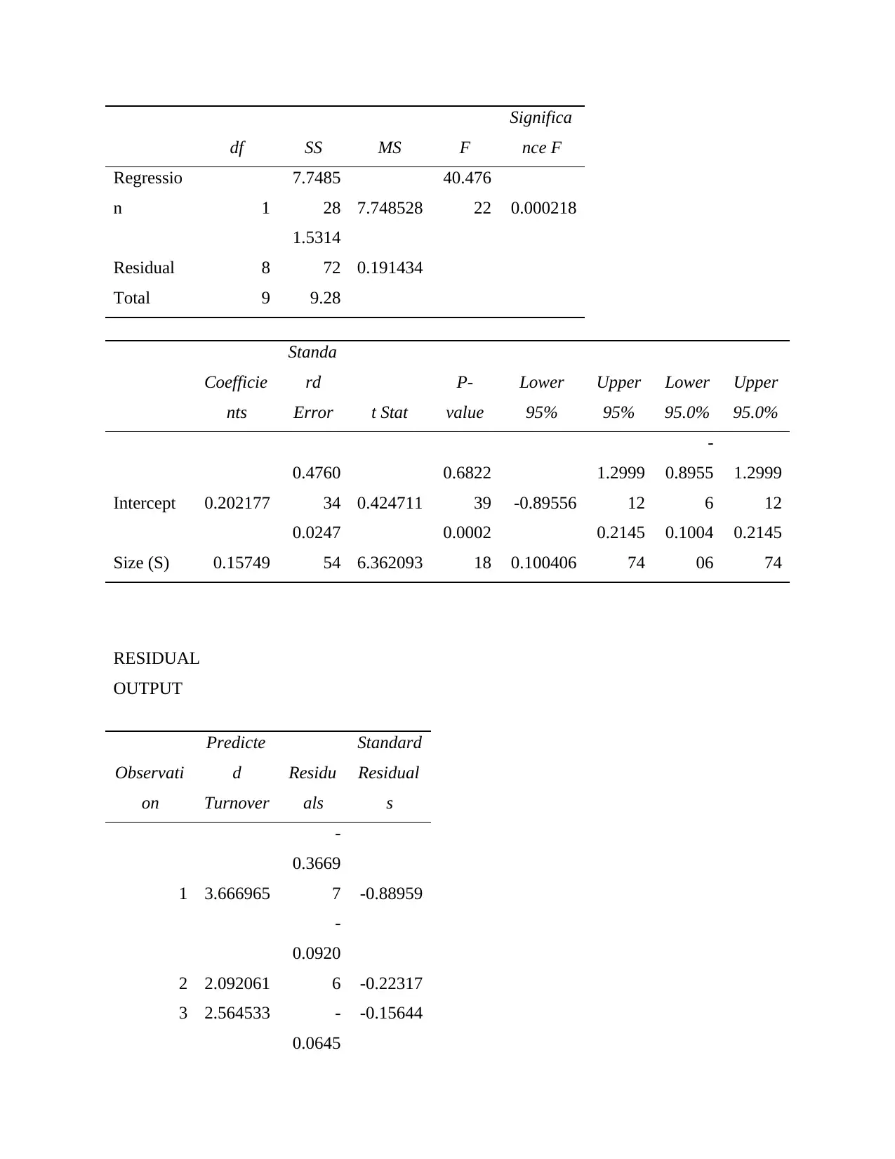
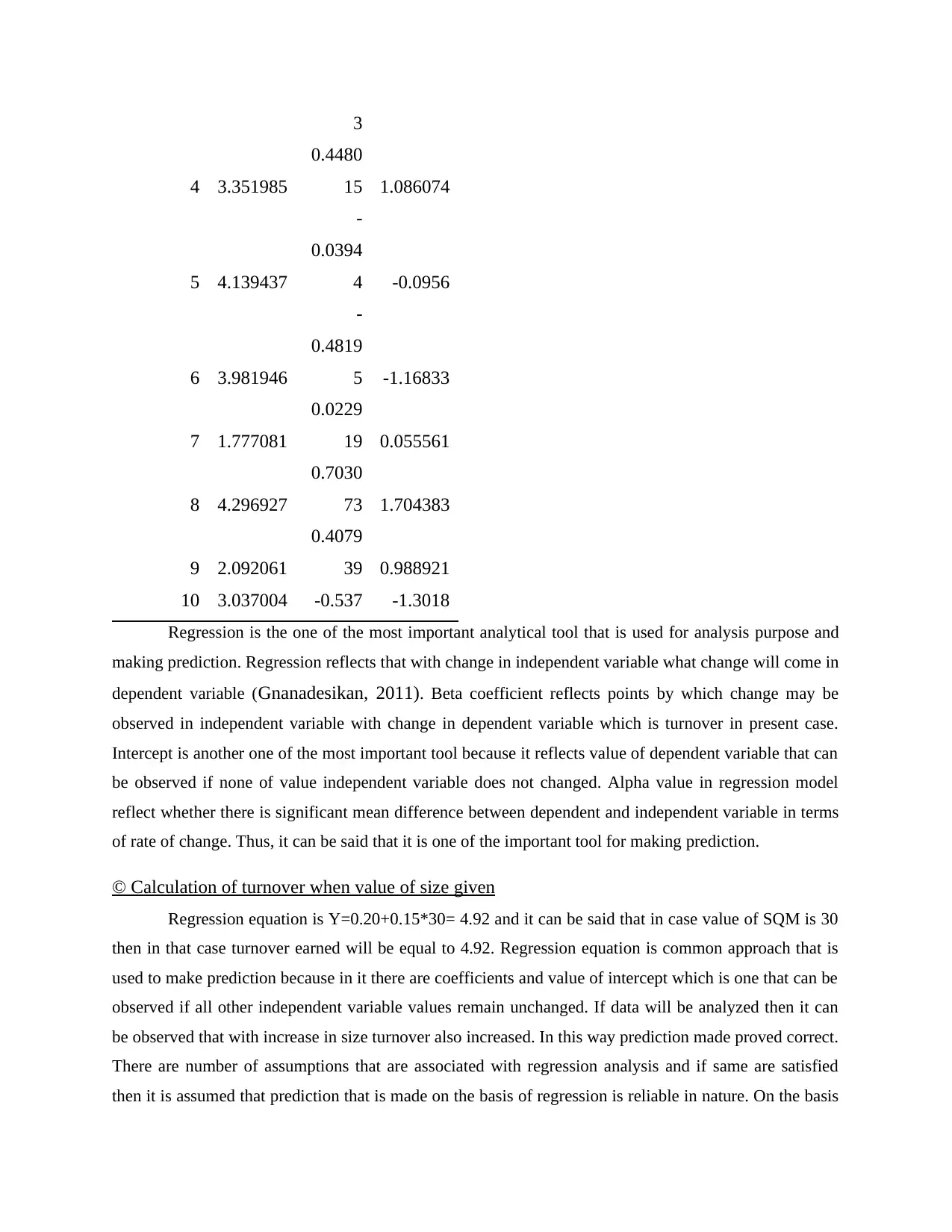
Regression is the one of the most important analytical tool that is used for analysis purpose and
making prediction. Regression reflects that with change in independent variable what change will come in
dependent variable (Gnanadesikan, 2011). Beta coefficient reflects points by which change may be
observed in independent variable with change in dependent variable which is turnover in present case.
Intercept is another one of the most important tool because it reflects value of dependent variable that can
be observed if none of value independent variable does not changed. Alpha value in regression model
reflect whether there is significant mean difference between dependent and independent variable in terms
of rate of change. Thus, it can be said that it is one of the important tool for making prediction.
© Calculation of turnover when value of size given
Regression equation is Y=0.20+0.15*30= 4.92 and it can be said that in case value of SQM is 30
then in that case turnover earned will be equal to 4.92. Regression equation is common approach that is
used to make prediction because in it there are coefficients and value of intercept which is one that can be
observed if all other independent variable values remain unchanged. If data will be analyzed then it can
be observed that with increase in size turnover also increased. In this way prediction made proved correct.
There are number of assumptions that are associated with regression analysis and if same are satisfied
then it is assumed that prediction that is made on the basis of regression is reliable in nature. On the basis
4 3.351985
0.4480
15 1.086074
5 4.139437
-
0.0394
4 -0.0956
6 3.981946
-
0.4819
5 -1.16833
7 1.777081
0.0229
19 0.055561
8 4.296927
0.7030
73 1.704383
9 2.092061
0.4079
39 0.988921
10 3.037004 -0.537 -1.3018
Regression is the one of the most important analytical tool that is used for analysis purpose and
making prediction. Regression reflects that with change in independent variable what change will come in
dependent variable (Gnanadesikan, 2011). Beta coefficient reflects points by which change may be
observed in independent variable with change in dependent variable which is turnover in present case.
Intercept is another one of the most important tool because it reflects value of dependent variable that can
be observed if none of value independent variable does not changed. Alpha value in regression model
reflect whether there is significant mean difference between dependent and independent variable in terms
of rate of change. Thus, it can be said that it is one of the important tool for making prediction.
© Calculation of turnover when value of size given
Regression equation is Y=0.20+0.15*30= 4.92 and it can be said that in case value of SQM is 30
then in that case turnover earned will be equal to 4.92. Regression equation is common approach that is
used to make prediction because in it there are coefficients and value of intercept which is one that can be
observed if all other independent variable values remain unchanged. If data will be analyzed then it can
be observed that with increase in size turnover also increased. In this way prediction made proved correct.
There are number of assumptions that are associated with regression analysis and if same are satisfied
then it is assumed that prediction that is made on the basis of regression is reliable in nature. On the basis
⊘ This is a preview!⊘
Do you want full access?
Subscribe today to unlock all pages.
Trusted by 1+ million students worldwide
1 out of 20
Related Documents


Your All-in-One AI-Powered Toolkit for Academic Success.
+13062052269
info@desklib.com
Available 24*7 on WhatsApp / Email
![[object Object]](/_next/static/media/star-bottom.7253800d.svg)
Unlock your academic potential
Copyright © 2020–2026 A2Z Services. All Rights Reserved. Developed and managed by ZUCOL.