Statistics for Management: Analysis of Income and Performance
VerifiedAdded on 2020/07/22
|22
|5114
|86
Report
AI Summary
This report provides a comprehensive analysis of statistical methods in management. It begins with an introduction to statistical concepts and their relevance, followed by a detailed examination of hypothesis testing applied to income levels in both public and private sectors. The report utilizes T-tests to compare income differences between men and women, presenting data through tables and charts to illustrate trends and variations. Further analysis includes the presentation of earnings-time charts and the calculation of annual growth rates to provide a clear understanding of income dynamics. The report also delves into data presentation using graphs and data analysis, exploring measures of central tendency and dispersion. Additionally, it covers the application of the Economic Order Quantity (EOQ) model, comparing it with actual costs. The final section presents bar and pie charts, analyzing the relationship between the number of bedrooms and prices in different locations, drawing conclusions on the presented data and providing a complete overview of the statistical techniques applied in management contexts.

STATISTICS FOR
MANAGEMENT
MANAGEMENT
Paraphrase This Document
Need a fresh take? Get an instant paraphrase of this document with our AI Paraphraser
TABLE OF CONTENTS
INTRODUCTION...........................................................................................................................1
TASK 1............................................................................................................................................1
(A) Hypothesis Testing based on income level in public industry........................................2
B) Presenting income level of man and women in the workplace in private industry...........3
C) Presenting Earnings – Time chart for each of the group ..................................................4
D) Producing annual growth rate ..........................................................................................4
TASK 2............................................................................................................................................6
2.1 Presentation of data through graph...................................................................................6
2.2 Presentation of data analysis ...........................................................................................7
B) Dispersion..........................................................................................................................9
2.3 Presenting report and interpretation.................................................................................9
SECTION B...................................................................................................................................10
2.4 Best fit line.....................................................................................................................10
TASK 3..........................................................................................................................................13
A) Presenting number of deliveries made in a particular period..........................................13
B) Outlining deliveries made in each round.........................................................................13
C) Defining EOQ..................................................................................................................13
D) Outlining comparison between EOQ and cost................................................................14
TASK 4..........................................................................................................................................16
4.1 Presentation of bar chart and pie chart by using data analysis.......................................16
4.2 Outlining relationship between number of bedrooms and different prices in Green street,
Church lane and Eton avenue...............................................................................................18
CONCLUSION..............................................................................................................................19
REFERENCES..............................................................................................................................20
INTRODUCTION
Statistics is a useful branch to show relations among variables to understand difference
with much ease by the statisticians. The present report deals with statistics in management and
highlights importance of statistical computation in various spheres of calculations by the
statistician. It discusses testing of hypothesis between two different sets of data to draw
meaningful conclusion with much ease. Moreover, calculations related to central tendencies such
as mean, mode is also done. Apart from this, standard deviation is also computed. ANOVA
technique is also drawn out to measure variability and EOQ model is also described to show how
stock should be purchased by the company to minimise overall cost.
TASK 1
1
⊘ This is a preview!⊘
Do you want full access?
Subscribe today to unlock all pages.
Trusted by 1+ million students worldwide
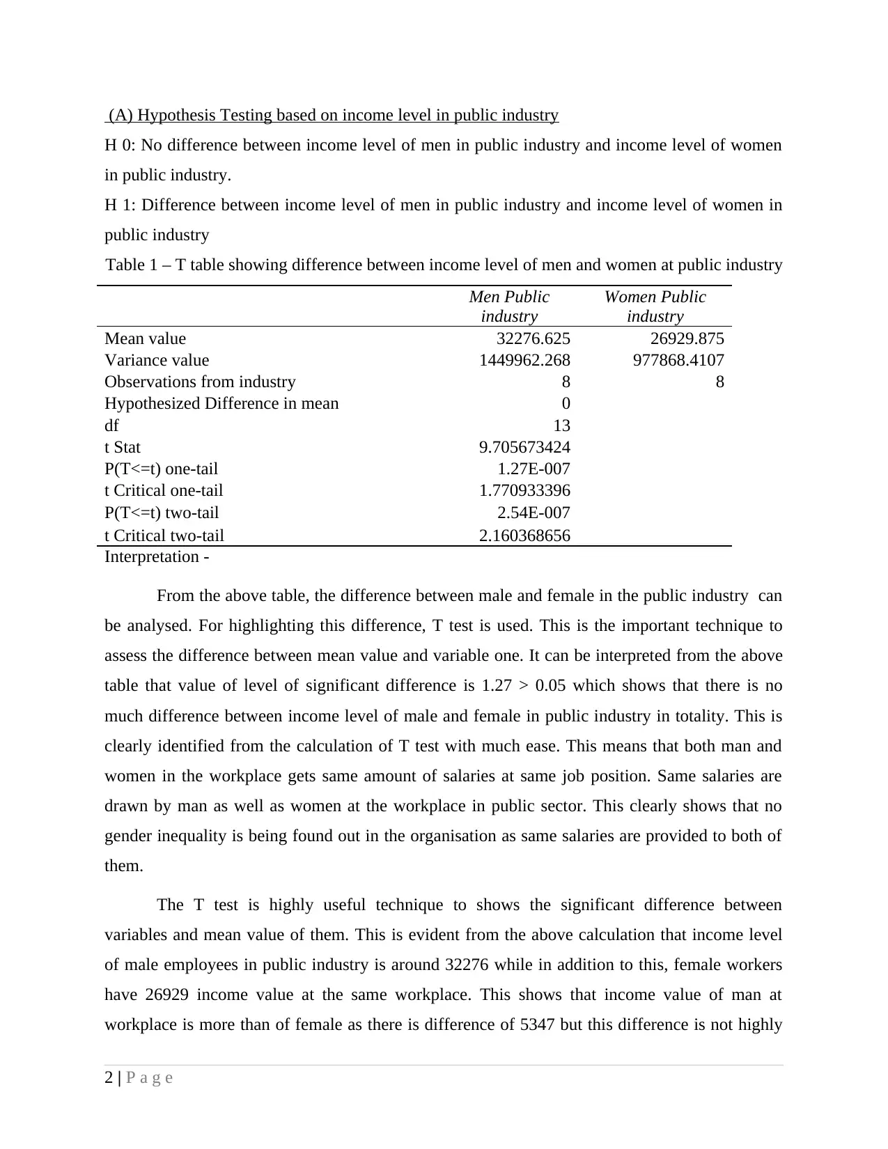
(A) Hypothesis Testing based on income level in public industry
H 0: No difference between income level of men in public industry and income level of women
in public industry.
H 1: Difference between income level of men in public industry and income level of women in
public industry
Table 1 – T table showing difference between income level of men and women at public industry
Men Public
industry
Women Public
industry
Mean value 32276.625 26929.875
Variance value 1449962.268 977868.4107
Observations from industry 8 8
Hypothesized Difference in mean 0
df 13
t Stat 9.705673424
P(T<=t) one-tail 1.27E-007
t Critical one-tail 1.770933396
P(T<=t) two-tail 2.54E-007
t Critical two-tail 2.160368656
Interpretation -
From the above table, the difference between male and female in the public industry can
be analysed. For highlighting this difference, T test is used. This is the important technique to
assess the difference between mean value and variable one. It can be interpreted from the above
table that value of level of significant difference is 1.27 > 0.05 which shows that there is no
much difference between income level of male and female in public industry in totality. This is
clearly identified from the calculation of T test with much ease. This means that both man and
women in the workplace gets same amount of salaries at same job position. Same salaries are
drawn by man as well as women at the workplace in public sector. This clearly shows that no
gender inequality is being found out in the organisation as same salaries are provided to both of
them.
The T test is highly useful technique to shows the significant difference between
variables and mean value of them. This is evident from the above calculation that income level
of male employees in public industry is around 32276 while in addition to this, female workers
have 26929 income value at the same workplace. This shows that income value of man at
workplace is more than of female as there is difference of 5347 but this difference is not highly
2 | P a g e
Paraphrase This Document
Need a fresh take? Get an instant paraphrase of this document with our AI Paraphraser
deviated. On the other hand, variance value of male is much than that of female which is
1449962 and 977868 of male and female respectively. Thus, income level of male is much
deviating than that of female at the workplace.
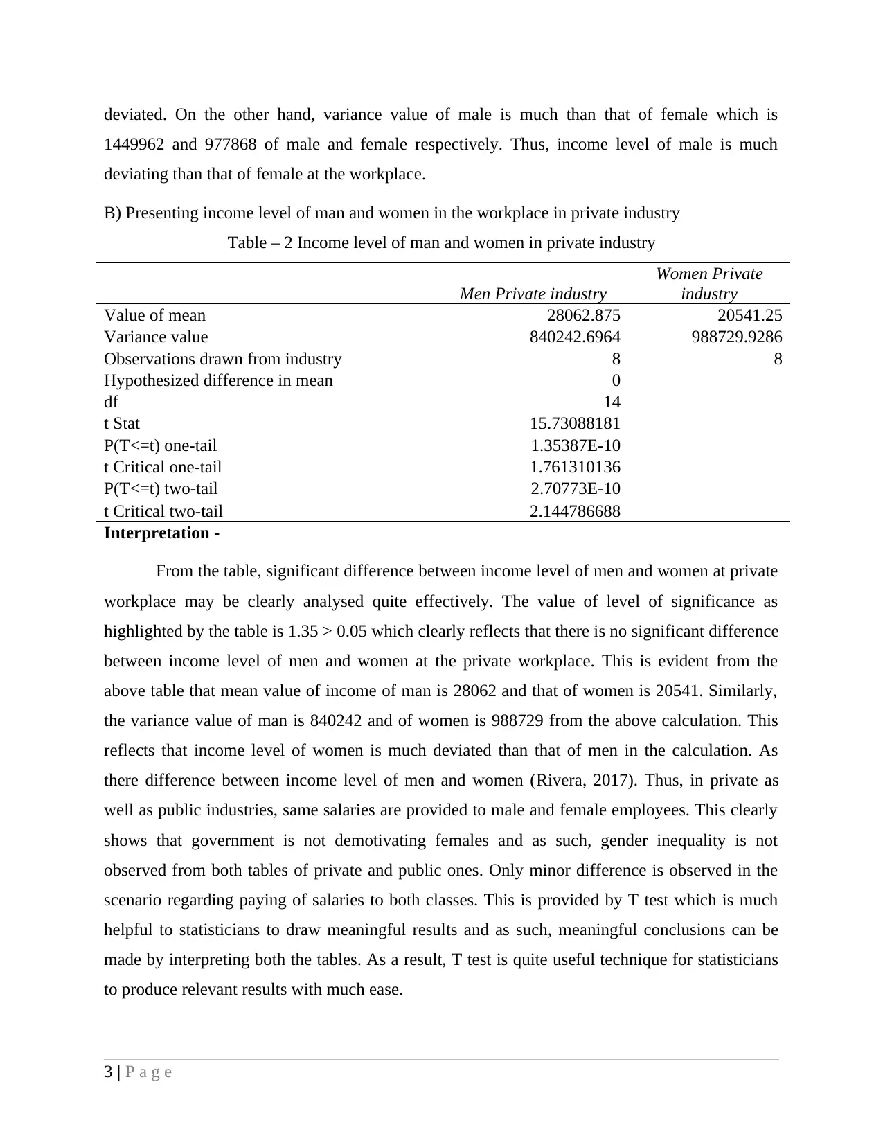
B) Presenting income level of man and women in the workplace in private industry
Table – 2 Income level of man and women in private industry
Men Private industry
Women Private
industry
Value of mean 28062.875 20541.25
Variance value 840242.6964 988729.9286
Observations drawn from industry 8 8
Hypothesized difference in mean 0
df 14
t Stat 15.73088181
P(T<=t) one-tail 1.35387E-10
t Critical one-tail 1.761310136
P(T<=t) two-tail 2.70773E-10
t Critical two-tail 2.144786688
Interpretation -
From the table, significant difference between income level of men and women at private
workplace may be clearly analysed quite effectively. The value of level of significance as
highlighted by the table is 1.35 > 0.05 which clearly reflects that there is no significant difference
between income level of men and women at the private workplace. This is evident from the
above table that mean value of income of man is 28062 and that of women is 20541. Similarly,
the variance value of man is 840242 and of women is 988729 from the above calculation. This
reflects that income level of women is much deviated than that of men in the calculation. As
there difference between income level of men and women (Rivera, 2017). Thus, in private as
well as public industries, same salaries are provided to male and female employees. This clearly
shows that government is not demotivating females and as such, gender inequality is not
observed from both tables of private and public ones. Only minor difference is observed in the
scenario regarding paying of salaries to both classes. This is provided by T test which is much
helpful to statisticians to draw meaningful results and as such, meaningful conclusions can be
made by interpreting both the tables. As a result, T test is quite useful technique for statisticians
to produce relevant results with much ease.
3 | P a g e
1449962 and 977868 of male and female respectively. Thus, income level of male is much
deviating than that of female at the workplace.
B) Presenting income level of man and women in the workplace in private industry
Table – 2 Income level of man and women in private industry
Men Private industry
Women Private
industry
Value of mean 28062.875 20541.25
Variance value 840242.6964 988729.9286
Observations drawn from industry 8 8
Hypothesized difference in mean 0
df 14
t Stat 15.73088181
P(T<=t) one-tail 1.35387E-10
t Critical one-tail 1.761310136
P(T<=t) two-tail 2.70773E-10
t Critical two-tail 2.144786688
Interpretation -
From the table, significant difference between income level of men and women at private
workplace may be clearly analysed quite effectively. The value of level of significance as
highlighted by the table is 1.35 > 0.05 which clearly reflects that there is no significant difference
between income level of men and women at the private workplace. This is evident from the
above table that mean value of income of man is 28062 and that of women is 20541. Similarly,
the variance value of man is 840242 and of women is 988729 from the above calculation. This
reflects that income level of women is much deviated than that of men in the calculation. As
there difference between income level of men and women (Rivera, 2017). Thus, in private as
well as public industries, same salaries are provided to male and female employees. This clearly
shows that government is not demotivating females and as such, gender inequality is not
observed from both tables of private and public ones. Only minor difference is observed in the
scenario regarding paying of salaries to both classes. This is provided by T test which is much
helpful to statisticians to draw meaningful results and as such, meaningful conclusions can be
made by interpreting both the tables. As a result, T test is quite useful technique for statisticians
to produce relevant results with much ease.
3 | P a g e
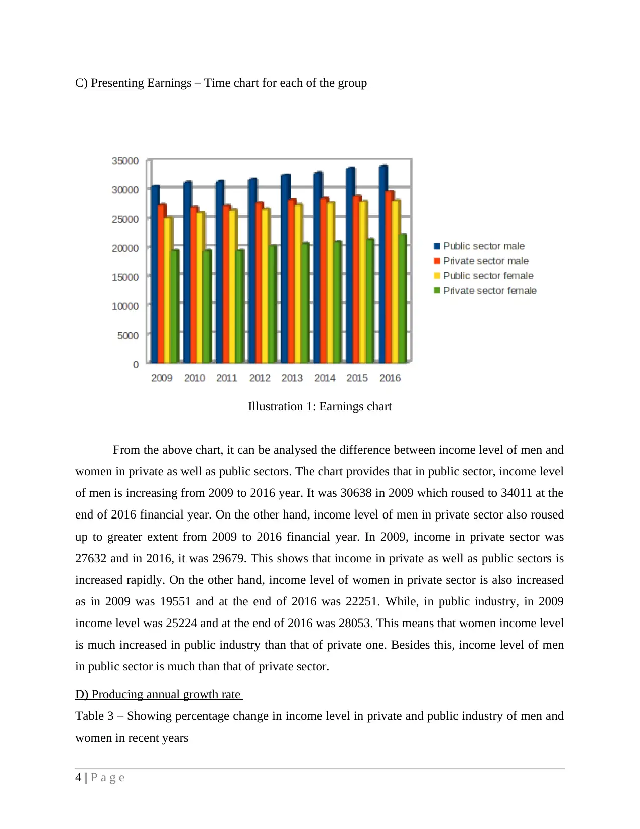
C) Presenting Earnings – Time chart for each of the group
From the above chart, it can be analysed the difference between income level of men and
women in private as well as public sectors. The chart provides that in public sector, income level
of men is increasing from 2009 to 2016 year. It was 30638 in 2009 which roused to 34011 at the
end of 2016 financial year. On the other hand, income level of men in private sector also roused
up to greater extent from 2009 to 2016 financial year. In 2009, income in private sector was
27632 and in 2016, it was 29679. This shows that income in private as well as public sectors is
increased rapidly. On the other hand, income level of women in private sector is also increased
as in 2009 was 19551 and at the end of 2016 was 22251. While, in public industry, in 2009
income level was 25224 and at the end of 2016 was 28053. This means that women income level
is much increased in public industry than that of private one. Besides this, income level of men
in public sector is much than that of private sector.
D) Producing annual growth rate
Table 3 – Showing percentage change in income level in private and public industry of men and
women in recent years
4 | P a g e
Illustration 1: Earnings chart
⊘ This is a preview!⊘
Do you want full access?
Subscribe today to unlock all pages.
Trusted by 1+ million students worldwide
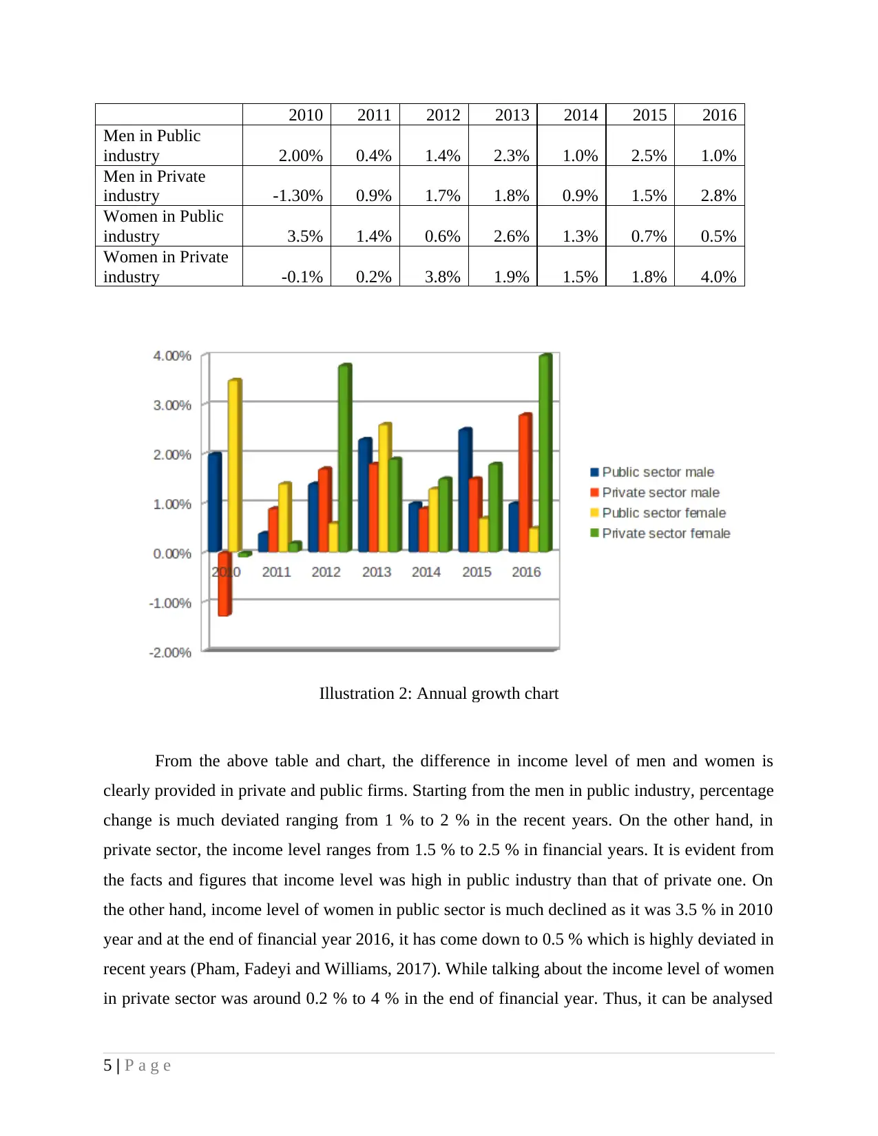
2010 2011 2012 2013 2014 2015 2016
Men in Public
industry 2.00% 0.4% 1.4% 2.3% 1.0% 2.5% 1.0%
Men in Private
industry -1.30% 0.9% 1.7% 1.8% 0.9% 1.5% 2.8%
Women in Public
industry 3.5% 1.4% 0.6% 2.6% 1.3% 0.7% 0.5%
Women in Private
industry -0.1% 0.2% 3.8% 1.9% 1.5% 1.8% 4.0%
From the above table and chart, the difference in income level of men and women is
clearly provided in private and public firms. Starting from the men in public industry, percentage
change is much deviated ranging from 1 % to 2 % in the recent years. On the other hand, in
private sector, the income level ranges from 1.5 % to 2.5 % in financial years. It is evident from
the facts and figures that income level was high in public industry than that of private one. On
the other hand, income level of women in public sector is much declined as it was 3.5 % in 2010
year and at the end of financial year 2016, it has come down to 0.5 % which is highly deviated in
recent years (Pham, Fadeyi and Williams, 2017). While talking about the income level of women
in private sector was around 0.2 % to 4 % in the end of financial year. Thus, it can be analysed
5 | P a g e
Illustration 2: Annual growth chart
Paraphrase This Document
Need a fresh take? Get an instant paraphrase of this document with our AI Paraphraser
that there is much difference between income level of men and women in both private and public
sectors. This can be seen from the chart that in income level of men at public sector is much
more than that of private sector. While, in case of women, private sector was much rapid than
that of other sector.
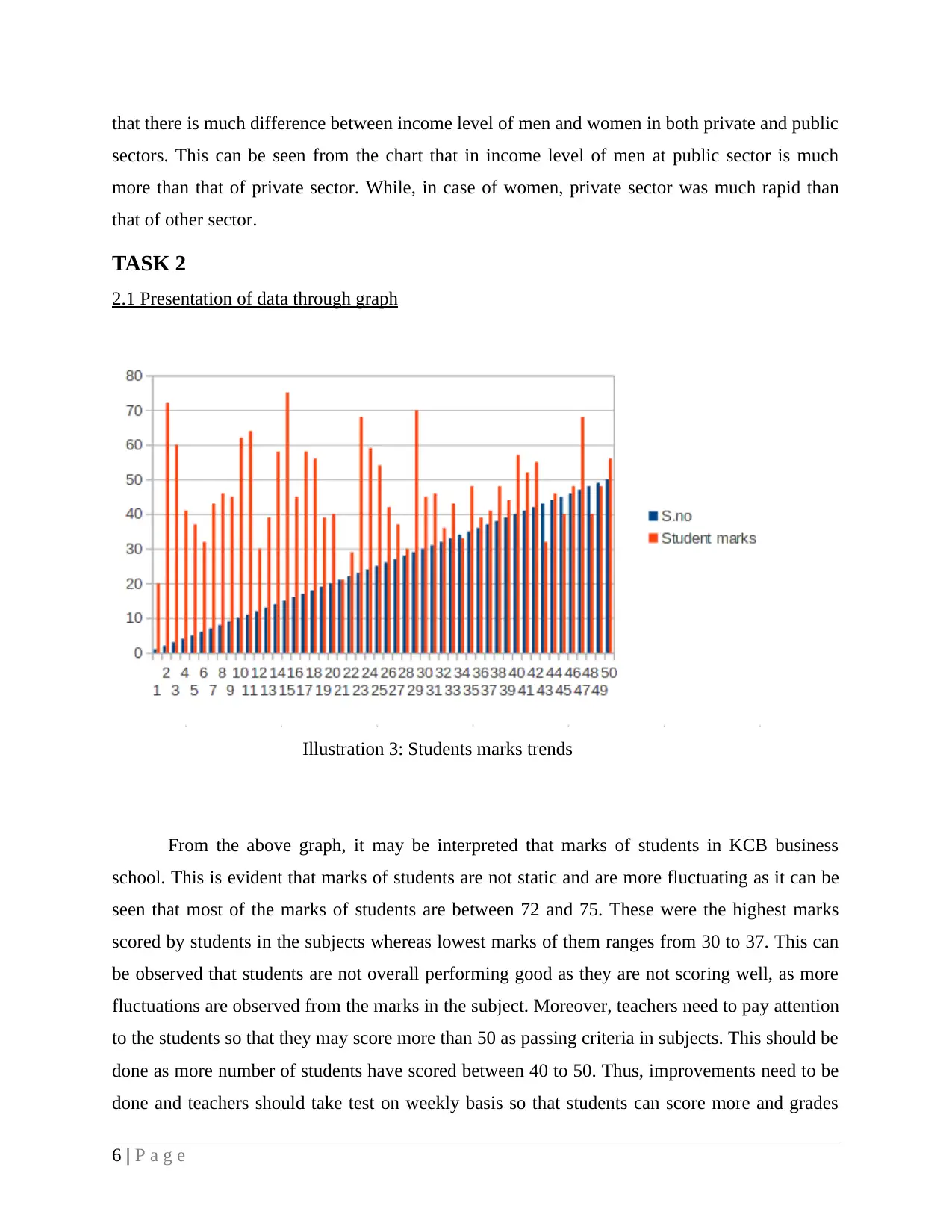
TASK 2
2.1 Presentation of data through graph
Illustration 3: Students marks trends
From the above graph, it may be interpreted that marks of students in KCB business
school. This is evident that marks of students are not static and are more fluctuating as it can be
seen that most of the marks of students are between 72 and 75. These were the highest marks
scored by students in the subjects whereas lowest marks of them ranges from 30 to 37. This can
be observed that students are not overall performing good as they are not scoring well, as more
fluctuations are observed from the marks in the subject. Moreover, teachers need to pay attention
to the students so that they may score more than 50 as passing criteria in subjects. This should be
done as more number of students have scored between 40 to 50. Thus, improvements need to be
done and teachers should take test on weekly basis so that students can score more and grades
6 | P a g e
sectors. This can be seen from the chart that in income level of men at public sector is much
more than that of private sector. While, in case of women, private sector was much rapid than
that of other sector.
TASK 2
2.1 Presentation of data through graph
Illustration 3: Students marks trends
From the above graph, it may be interpreted that marks of students in KCB business
school. This is evident that marks of students are not static and are more fluctuating as it can be
seen that most of the marks of students are between 72 and 75. These were the highest marks
scored by students in the subjects whereas lowest marks of them ranges from 30 to 37. This can
be observed that students are not overall performing good as they are not scoring well, as more
fluctuations are observed from the marks in the subject. Moreover, teachers need to pay attention
to the students so that they may score more than 50 as passing criteria in subjects. This should be
done as more number of students have scored between 40 to 50. Thus, improvements need to be
done and teachers should take test on weekly basis so that students can score more and grades
6 | P a g e
may be enhanced quite effectively (Artikis, 2017). By applying this tactic, students' performance
may be increased up to greater extent in the best possible way.
Furthermore, concentration power of students should also be enhanced so that they may
be able to perform well in the subjects and grades may be increased as well. This way students
can be enhanced by asking questions in the middle of classes to test their concentration level and
as such, they can be helped up to great extent to maximise grades. Apart from this, students need
to get organised their work on time so that proper studies can be attained within time. This
ensures that they are committed to time table so that studies are finished on time. Students should
write notes of every lectures taught in the class so that they may be able to learn quickly and as
such, teachers should laid emphasis so that they may write notes in the class. Apart from
teachers, parents should also concentrate on their children so that they perform well and grades
may be overall enhanced and they all may get more than 50 marks in the subjects.
2.2 Presentation of data analysis
Serial number
Scores of
students
1 20
2 72
3 60
4 41
5 37
6 32
7 43
8 46
9 45
10 62
11 64
12 30
13 39
14 58
15 75
16 45
17 58
18 56
19 39
20 40
21 21
7 | P a g e
⊘ This is a preview!⊘
Do you want full access?
Subscribe today to unlock all pages.
Trusted by 1+ million students worldwide
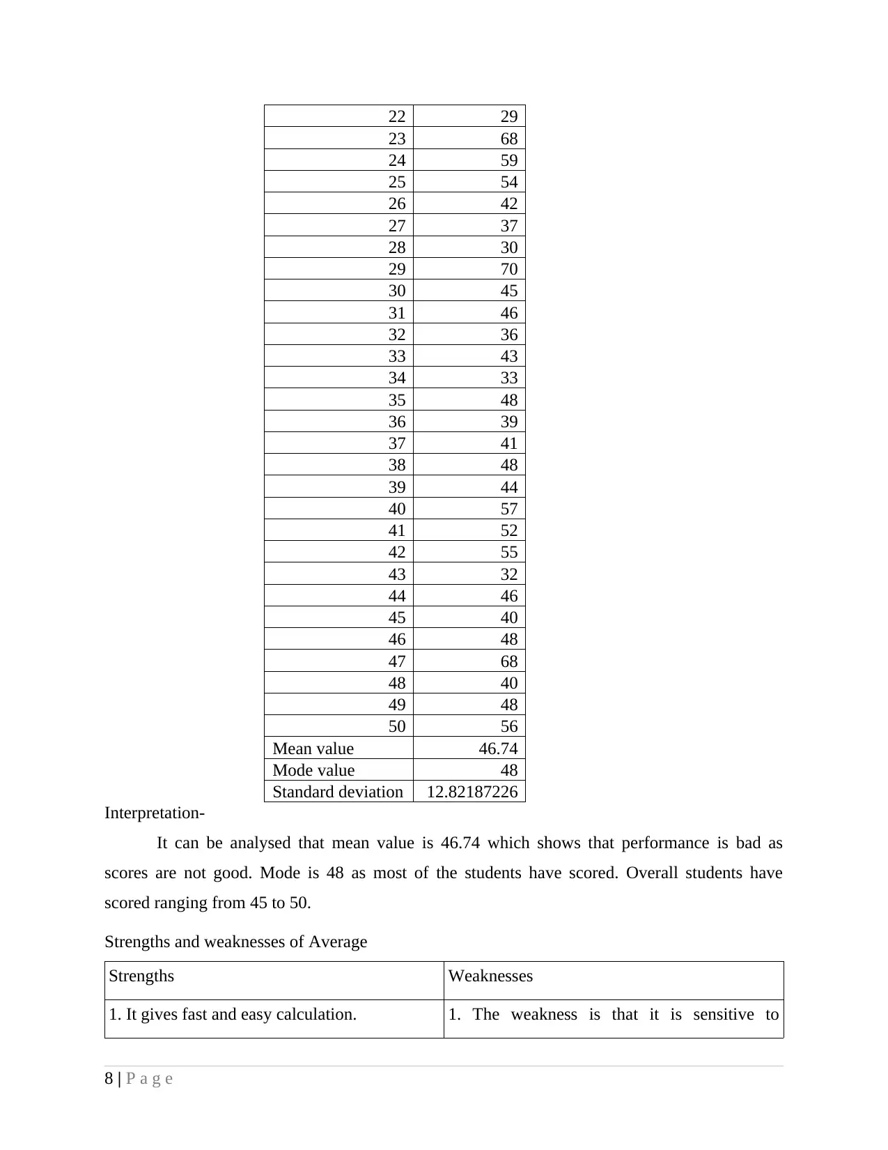
22 29
23 68
24 59
25 54
26 42
27 37
28 30
29 70
30 45
31 46
32 36
33 43
34 33
35 48
36 39
37 41
38 48
39 44
40 57
41 52
42 55
43 32
44 46
45 40
46 48
47 68
48 40
49 48
50 56
Mean value 46.74
Mode value 48
Standard deviation 12.82187226
Interpretation-
It can be analysed that mean value is 46.74 which shows that performance is bad as
scores are not good. Mode is 48 as most of the students have scored. Overall students have
scored ranging from 45 to 50.
Strengths and weaknesses of Average
Strengths Weaknesses
1. It gives fast and easy calculation. 1. The weakness is that it is sensitive to
8 | P a g e
Paraphrase This Document
Need a fresh take? Get an instant paraphrase of this document with our AI Paraphraser
extreme values and as suich, median can be
beneficial in such circumstances.
Strengths and weaknesses of Mode
Strengths Weaknesses
1. It gives most repetitive value from the data
set and is helpful when data is large enough.
2. It is more useful in qualitative data than
quantitative one.
1. It is unsuitable for smaller data and it cannot
be defined clearly in smaller set of data.
2. Mode is not suitable for further calculations
in further analysis.
B) Dispersion
The central tendency does not provide variable information in the data. As it has certain
limitations which is overcome by measures of dispersion (LESSON 4 MEASURES OF
DISPERSION). It is relative term which provides how value scatters from each other in the
average value and in a distribution. This means that more the deviation between them, better for
company as it provides reliable information of the average. In above calculation, standard
deviation comes out to be 12 which is moderately deviate from mean value. As such, it is
complex to predict marks of the students. As a result, measures of dispersion is essential tool to
make enhanced decisions.
2.3 Presenting report and interpretation
To
The Director of KCB School
Subject: Overall performance of students in class
Mean, mode interpretation
The mean value is 46.7 and that of mode is 48. On an average, more students have scored 46
marks while 48 is scored more number of times than mean 46.7.
Standard deviation
The value of standard deviation is 12.82 which is moderate and as such, it is difficult to make
prediction in future marks of students as much deviation is prevailing.
9 | P a g e
Ways can be adopted to compare between subjects
To compare subjects effectively, T test can be used which provides clear significant difference
between independent variables from the data. Moreover, another way is by using ANOVA
technique which is used to determine difference between group means quite effectively. This
technique will be helpful for comparison purpose among the data.
Ways to measure association
For measuring association, correlation method should be used so that relation between two
subjects can be made easily by the individual with much ease. Chi square can also be used to
find out relationship among different variables from the data set quite effectively.
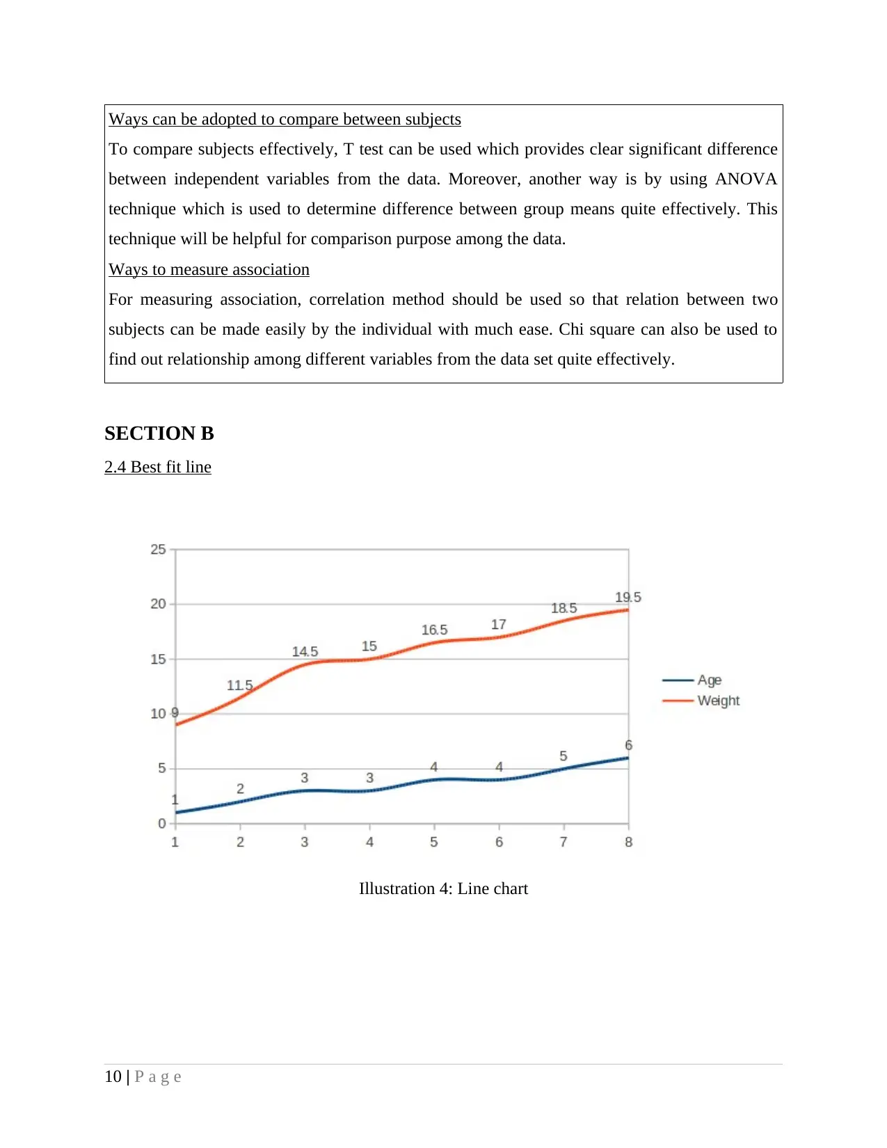
SECTION B
2.4 Best fit line
10 | P a g e
Illustration 4: Line chart
To compare subjects effectively, T test can be used which provides clear significant difference
between independent variables from the data. Moreover, another way is by using ANOVA
technique which is used to determine difference between group means quite effectively. This
technique will be helpful for comparison purpose among the data.
Ways to measure association
For measuring association, correlation method should be used so that relation between two
subjects can be made easily by the individual with much ease. Chi square can also be used to
find out relationship among different variables from the data set quite effectively.
SECTION B
2.4 Best fit line
10 | P a g e
Illustration 4: Line chart
⊘ This is a preview!⊘
Do you want full access?
Subscribe today to unlock all pages.
Trusted by 1+ million students worldwide
1 out of 22
Related Documents


Your All-in-One AI-Powered Toolkit for Academic Success.
+13062052269
info@desklib.com
Available 24*7 on WhatsApp / Email
![[object Object]](/_next/static/media/star-bottom.7253800d.svg)
Unlock your academic potential
Copyright © 2020–2026 A2Z Services. All Rights Reserved. Developed and managed by ZUCOL.