Statistics Assignment: Probability, Distributions, and Analysis

This statistics assignment solution covers fundamental concepts including probability and frequency distributions, coin tossing scenarios, and probability calculations. It delves into real-world applications using population data from Australia to calculate probabilities, followed by an analysis of labor time using confidence intervals and standard errors. The assignment concludes with a hypothesis testing problem, assessing customer travel distances for a store's advertising strategy, utilizing t-tests to determine whether the average customer lives within a certain radius. This comprehensive solution provides detailed explanations and calculations for each question, including the use of standard deviations, mean values, and confidence levels, demonstrating a strong understanding of statistical principles.

Running head: STATISTICS
Statistics
Name of the Student:
Name of the University:
Author’s note:

1STATISTICS
Table of Contents
Question 1..................................................................................................................................2
1.a) Probability Distribution:.................................................................................................2
1.b) Frequency Distribution:..................................................................................................2
1.c) Coin Tossing:..................................................................................................................3
1.d) Calculation of Probability:..............................................................................................3
Question 2..................................................................................................................................3
Question 3..................................................................................................................................4
3.a)..........................................................................................................................................4
3.b).........................................................................................................................................5
References:.................................................................................................................................7
a.

2STATISTICS
Question 1.
1.a) Probability Distribution:
A probability distribution is a statistical function (f ( x)¿ that indicates all the probable and
likelihood values that a random variable can take within a defined range.
The probability distribution is divided in two ways that are-
Discrete Probability Distribution: It is the probabilistic properties of observable pre-
assigned values. The observable values may either be finite or countably infinite (discrete)
probability distribution. A limited number of probable observations generates discrete
probability distribution. A discrete random variable could be related with a non-zero
probability.
Example: The distribution of errors found per page of a book.
Continuous Probability Distribution: A continuous probability distribution refers the
probabilities of probable values of a continuous random variable. A set of infinite and
uncountable continuous probable values create continuous probability distribution.
Example: The distribution of heights of adult males.
1.b) Frequency Distribution:
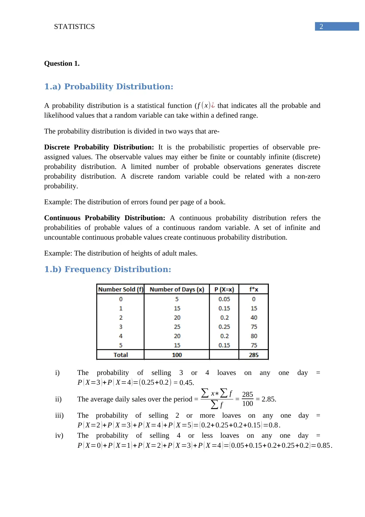
i) The probability of selling 3 or 4 loaves on any one day =
P ( X=3 ) + P ( X=4 ) =(0.25+0.2) = 0.45.
ii) The average daily sales over the period = ∑ x∗∑ f
∑ f = 285
100 = 2.85.
iii) The probability of selling 2 or more loaves on any one day =
P ( X=2 )+ P ( X =3 ) + P ( X=4 )+ P ( X =5 )= ( 0.2+ 0.25+0.2+0.15 ) =0.8 .
iv) The probability of selling 4 or less loaves on any one day =
P ( X=0 ) + P ( X=1 ) + P ( X=2 ) + P ( X =3 ) + P ( X =4 ) = ( 0.05+0.15+ 0.2+0.25+0.2 ) =0.85 .

3STATISTICS
1.c) Coin Tossing:
A coin is tossed twice. The events of flipping the coin two times are independent to
each other. The sample space of two tosses is: Ω = {HH, HT, TH, TT}
The probability of each individual event = P(HH) = P(HT) = P(TH) = P(TT) = 1
4 =0.25 (Due
to independence) (Dudley, 2018).
i) The probability of a head on the first toss = P(HH) + P(HT) = 0.25+0.25 = 0.5
ii) The probability of getting a tail on the second toss given a head on the first toss =
P(HT)= 0.25
iii) The probability of getting two tails in two throws = P (TT) = 0.25.
iv) The probability of getting a tail in first toss and a head on the second toss = P
(TH) = 0.25.
v) The probability of getting a tail on the first and a head on the second or a head on
the first and a tail on the second = P (TH) + P (HT) = (0.25+0.25) = 0.5.
vi) The probability of at least one head on the first two tosses = P (HT) + P (HT) +
P(HH) = (0.25+0.25+0.25) = 0.75.
1.d) Calculation of Probability:
The mean value of sales of apples is 5000.
The value of standard deviation of sales of apples is 600.
Therefore,
 The probability of sales that will be greater than 5600 apples =
P ( X >5600) = P ( X – 5000 > 5600-5000) = P ( X -μ>600) = P ( X−μ
600 > 600
600 ) = P ( X−μ
σ >1) =
P (Z>1) = 0.1587 (Ross, 2014).
 The probability of sales that will be less than 5240 apples =
P ( X <5240) = P ( X – 5000 < 5240-5000) = P ( X -μ<240) = P ( X−μ
600 < 240
600 ) = P ( X−μ
σ <0.4)
= P (Z<0.4) = 0.6554.
 The probability of sales that will be less than 4400 apples =
P ( X <4400) = P ( X – 5000 < 4400-5000) = P ( X -μ < -600) = P ( X−μ
600 < 60 0
−600 ) = P (
X−μ
σ <−1) = P (Z<-1) = 0.1587.

4STATISTICS
Question 2.
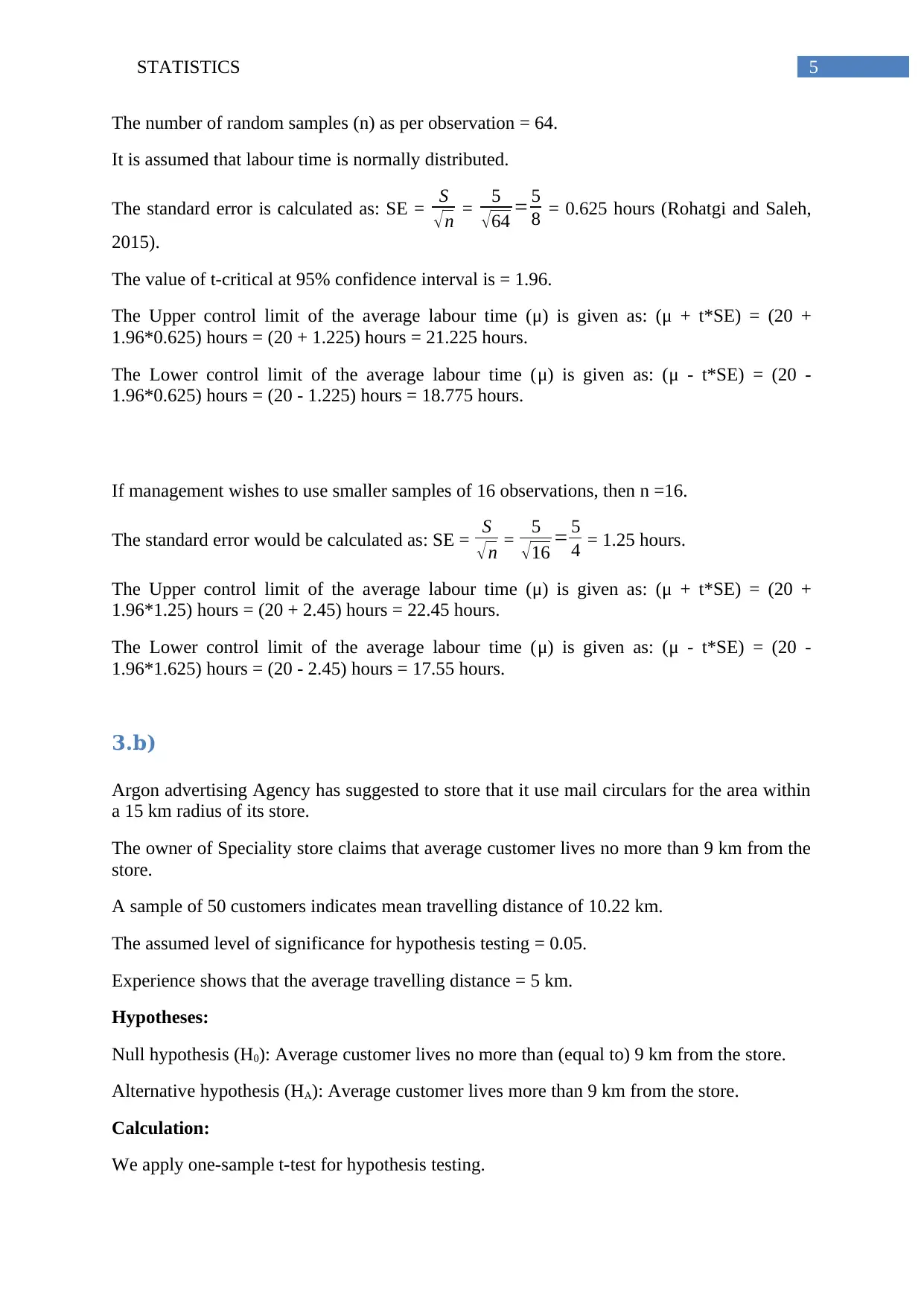
Table 1: Table of population distribution of males and females of different age groups in Australia in the time period
2001 to 2017
(Source:
http://www.abs.gov.au/AUSSTATS/abs@.nsf/DetailsPage/3101.0Jun%202017?
OpenDocument)
The latest time period is undertaken as 2001 to 2017.
 The probability that any person selected at random method from the population is
male = Total number of males
Total population =¿ 2642593
5324232 = 0.4963.
 The probability that any person selected at random from the population is aged
between 55 and 64 = The number of people of age 55 ¿ 64 ¿
Total number of people =
1021538
5324232 = 0.191866.
 The joint probability that any person selected at random from the population is a
female and aged between 15 and 24 =
The number of females whose ages are between 15∧24
Total population = 275556
5324232 = 0.051755.
 The probability that any person selected at random from the population is 55 or over =
The number of people of the age 55 ¿ 64+The number of people of the age 65∧¿ ¿
Total population
= (1021538+1375730)
5324232 = 2397268
5324232 = 0.450256.
Question 3.
3.a)
The average labour time (μ) to deliver a product is 20 hours.
The standard deviation (S) of labour time to deliver a product is 5 hours.

5STATISTICS
The number of random samples (n) as per observation = 64.
It is assumed that labour time is normally distributed.
The standard error is calculated as: SE = S
√ n = 5
√64 = 5
8 = 0.625 hours (Rohatgi and Saleh,
2015).
The value of t-critical at 95% confidence interval is = 1.96.
The Upper control limit of the average labour time (μ) is given as: (μ + t*SE) = (20 +
1.96*0.625) hours = (20 + 1.225) hours = 21.225 hours.
The Lower control limit of the average labour time (μ) is given as: (μ - t*SE) = (20 -
1.96*0.625) hours = (20 - 1.225) hours = 18.775 hours.
If management wishes to use smaller samples of 16 observations, then n =16.
The standard error would be calculated as: SE = S
√n = 5
√16 = 5
4 = 1.25 hours.
The Upper control limit of the average labour time (μ) is given as: (μ + t*SE) = (20 +
1.96*1.25) hours = (20 + 2.45) hours = 22.45 hours.
The Lower control limit of the average labour time (μ) is given as: (μ - t*SE) = (20 -
1.96*1.625) hours = (20 - 2.45) hours = 17.55 hours.
3.b)
Argon advertising Agency has suggested to store that it use mail circulars for the area within
a 15 km radius of its store.
The owner of Speciality store claims that average customer lives no more than 9 km from the
store.
A sample of 50 customers indicates mean travelling distance of 10.22 km.
The assumed level of significance for hypothesis testing = 0.05.
Experience shows that the average travelling distance = 5 km.
Hypotheses:
Null hypothesis (H0): Average customer lives no more than (equal to) 9 km from the store.
Alternative hypothesis (HA): Average customer lives more than 9 km from the store.
Calculation:
We apply one-sample t-test for hypothesis testing.

6STATISTICS
Sample mean (μ) of distance of 50 customers = 9 km.
Population mean ( X ) distance = 10.22 km.
Standard deviation (S) in terms of experience = 5 km.
Number of samples (n) = 50.
Standard error of distance = SE = S
√ n = 5
√50 =¿ 0.707 hours.
The level of significance = 0.05.
The t-statistic at 5% level of significance = 1.96.
The calculated t-statistic =
( X−μ)
S
√n
=
(10.22−9)
5
√50
= 1.22
0.707 = 1.7253.
Decision Making:
As, tcric > tcal (1.7253<1.96), therefore, we cannot reject the null hypothesis at 5% level of
significance.
It could be concluded that average customer lives no more than 9 km. from the store with 5%
probability (Zhao, 2015).
Hence, the claim of Argon’s representative is found to be true.

7STATISTICS
References:
Dudley, R. M. (2018). Real analysis and probability. CRC Press.
Rohatgi, V. K., & Saleh, A. M. E. (2015). An introduction to probability and statistics. John
Wiley & Sons.
Ross, S. M. (2014). Introduction to probability models. Academic press.
Zhao, Y. (2015). Data mining techniques.