Statistics for Analytical Decisions Assignment - Stock Market Analysis

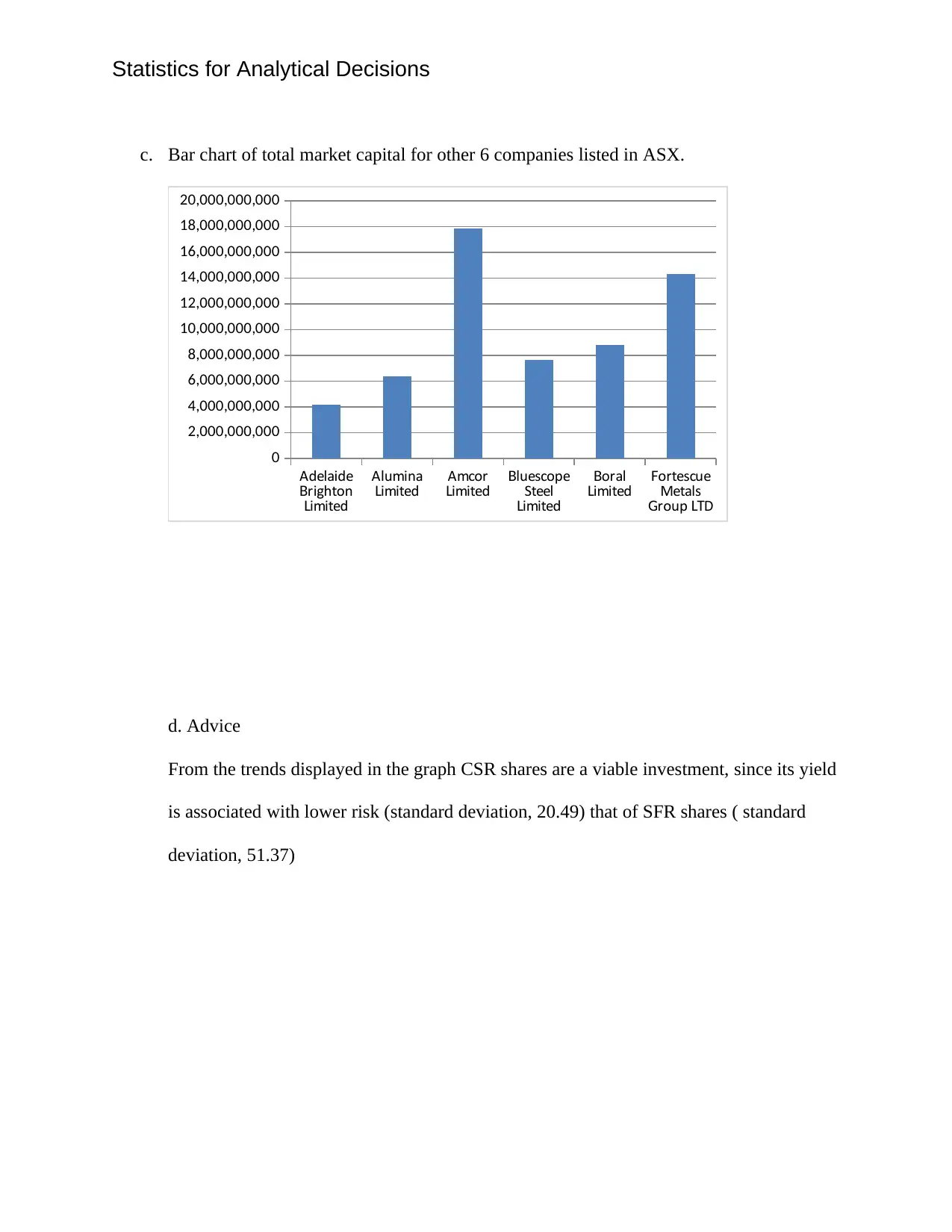
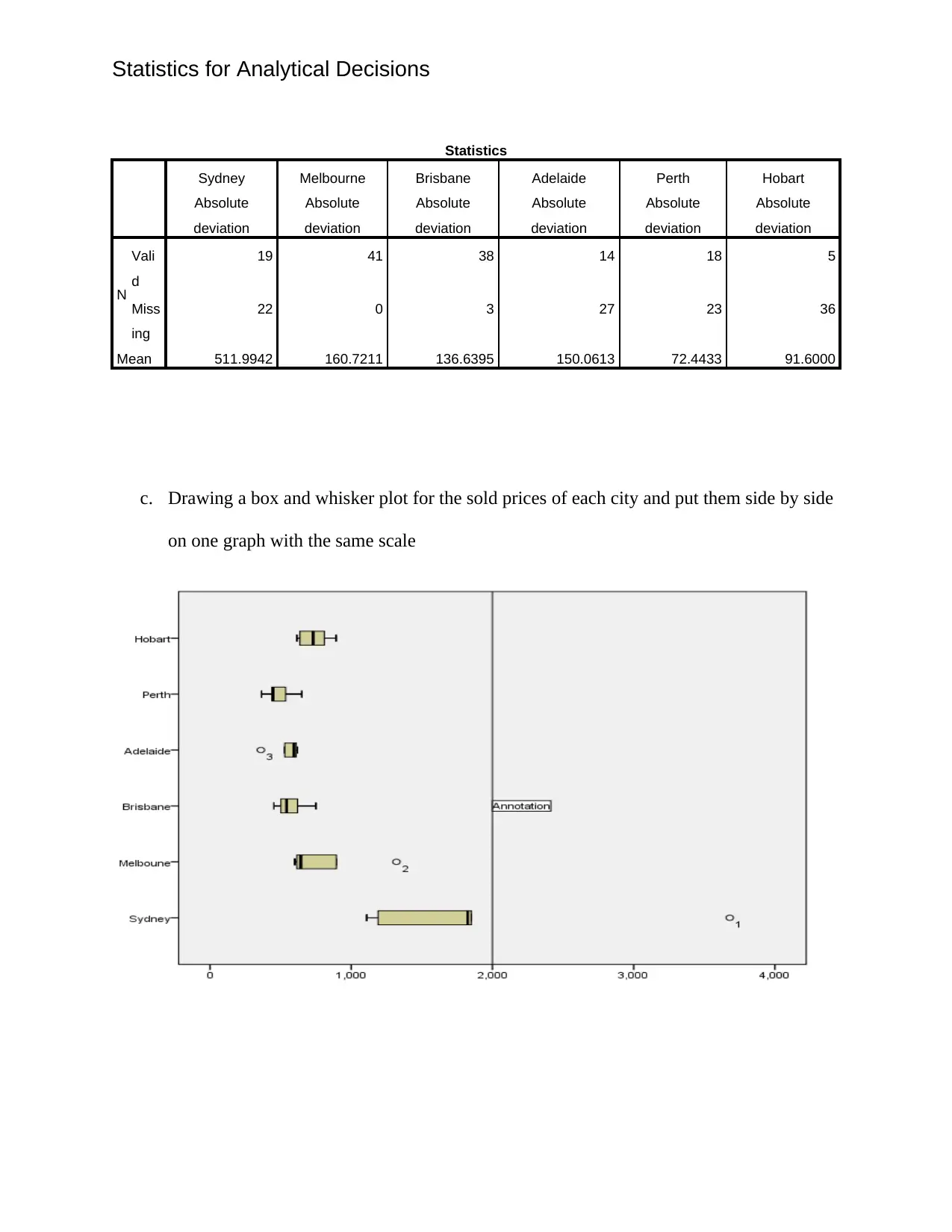
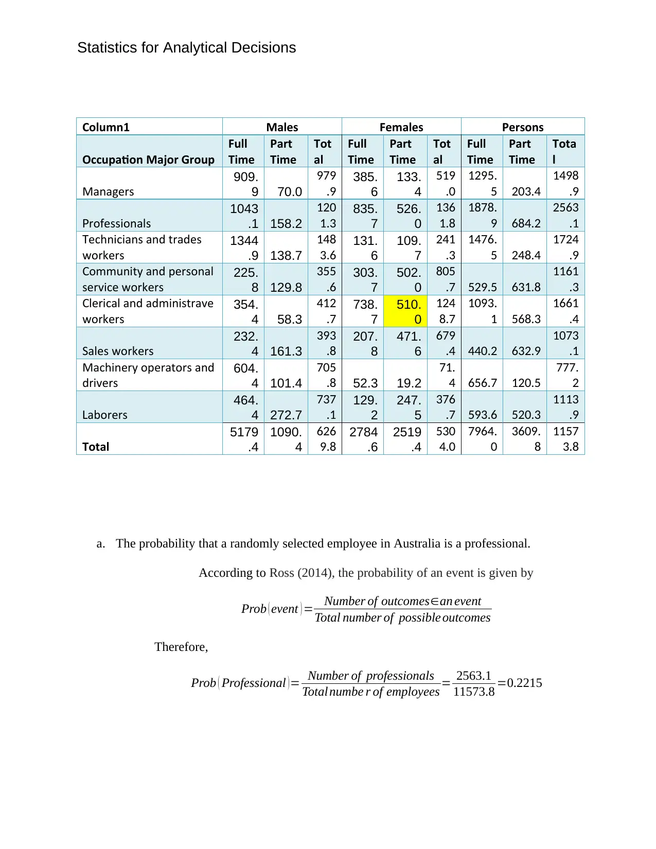
This statistics assignment presents a comprehensive analysis of various datasets, including Australian stock market data (CSR and SFR), apartment prices, and absenteeism from work. The assignment involves constructing stem-and-leaf plots, histograms, and bar charts to visualize data. It requires the calculation of probabilities, means, medians, standard deviations, and confidence intervals. The analysis extends to normality tests, rainfall data, and absenteeism data, with interpretations of statistical results. The assignment covers topics such as probability calculations, normality tests, and the construction of confidence intervals. The student analyzes stock market trends, apartment prices, and absenteeism data, providing interpretations and conclusions based on the statistical findings. The assignment utilizes software such as SPSS and Excel for statistical computations and data visualization.

Statistics for Analytical Decisions
Statistical Analysis Paper
Student’s Name
Institution Affiliation

Statistics for Analytical Decisions
Question One
Data; from Australia stock market
a. Tables of the quarterly opening price values of CSR and the other for SFR
CSR imitedL
Opening Price
Beginning of Yearly
Quarter
2008 200
9
201
0
201
1
2012 2013 2014 2015 2016 2017
anuaryJ 22.1 4.42 7.84 5.37 53.3
1
52.9
5
62.0
4
49.3 29.8
2
36.8
2
April 18 3.9 7.74 4.67 52.2 49.3
2
66.4
3
37.7
4
33.6
5
37.7
ulyJ 13.3
8
7.38 4.57 5.28 47.6
3
45.3
7
63.7 38.8
3
32.8
1
37.7
2
ctoberO 14 7.15 5.6 6.4 52.7
1
58.2 44.7
7
30.0
5
41.2
8
48.3
9
S R imitedF L
Opening Price
Beginning of Yearly
Quarter
200
8
2009 201
0
201
1
2012 2013 2014 2015 2016 2017
anuaryJ 37.4
6
31.4
2
52.8
3
57.5
7
57.2
8
115.7
5
122.4
1
131.8
6
139.2
3
144.4
5
April 34.6
6
28.5
2
51.9
9
59.5
8
71.1
6
138.6
9
123.4
2
136.1
1
148.7
8
173.1
3
ulyJ 34.2
9
39.3
5
45.5
4
59.4 78.8
8
113.4
6
127.5
7
141.8
5
159.3
4
207.5
ctoberO 31.2
1
42.7
3
47.4
7
49.2 88.2
7
109.4
9
127.8
7
152.5 146.6
8
191.7

Statistics for Analytical Decisions
Stem and leaf display
CSR Stem-and-Leaf Plot
Frequency Stem & Leaf
12.00 0 . 344455567777
3.00 1 . 348
2.00 2 . 29
8.00 3 . 02367778
7.00 4 . 1457899
5.00 5 . 22238
3.00 6 . 236
Stem width: 10.00
Each leaf: 1 case(s)
SFR Stem-and-Leaf Plot
Frequency Stem & Leaf
11.00 0 . 23333334444
9.00 0 . 555555778
15.00 1 . 011222233334444
4.00 1 . 5579
1.00 2 . 0
Stem width: 100.00
Each leaf: 1 case(s)

Statistics for Analytical Decisions
b. Histograms

Statistics for Analytical Decisions
c. Bar chart of total market capital for other 6 companies listed in ASX.
Adelaide
rightonB imitedL
Alumina
imitedL Amcor
imitedL luescopeB Steel
imitedL
oralB
imitedL ortescueF Metals
roup DG LT
0
2,000,000,000
4,000,000,000
6,000,000,000
8,000,000,000
10,000,000,000
12,000,000,000
14,000,000,000
16,000,000,000
18,000,000,000
20,000,000,000
d. Advice
From the trends displayed in the graph CSR shares are a viable investment, since its yield
is associated with lower risk (standard deviation, 20.49) that of SFR shares ( standard
deviation, 51.37)

Statistics for Analytical Decisions
Question Two
Data: The prices of apartments with 2 bedrooms and 2 bathrooms sold between January and July
of 2018 in Australian state capital city centers.
a. Computation of Mean, Median, first Quartile and third Quartile of sold price for each
city. These were statistics were computed on SPSS
Statistics
Melbourne Brisbane Adelaide Perth Hobart Sydney
N Valid 41 38 14 18 5 19
Missing 0 3 27 23 36 22
Mean 733.171 572.05 650.143 506.83 737.00 1778.11
Median 650.000 518.50 605.000 480.00 730.00 1810.00
Percentiles
25 600.000 448.75 518.750 440.00 626.00 1190.00
50 650.000 518.50 605.000 480.00 730.00 1810.00
75 795.500 650.00 699.500 537.50 851.50 2300.00
b. Computation of Standard deviation, Mean absolute deviation and range of sold price for
each city. These were statistics were computed on SPSS
Statistics
Melbourne Brisbane Adelaide Perth Hobart Sydney
N Valid 41 38 14 18 5 19
Missing 0 3 27 23 36 22
Std. Deviation 240.4076 173.076 247.8296 103.290 116.831 674.212
Range 1197.0 665 1055.0 450 278 2740
The means in the table below are the means absolute deviations of the sold price for each
city. These were statistics were computed on SPSS

Statistics for Analytical Decisions
Statistics
Sydney
Absolute
deviation
Melbourne
Absolute
deviation
Brisbane
Absolute
deviation
Adelaide
Absolute
deviation
Perth
Absolute
deviation
Hobart
Absolute
deviation
N
Vali
d
19 41 38 14 18 5
Miss
ing
22 0 3 27 23 36
Mean 511.9942 160.7211 136.6395 150.0613 72.4433 91.6000
c. Drawing a box and whisker plot for the sold prices of each city and put them side by side
on one graph with the same scale

Statistics for Analytical Decisions
d. Comment on the 2 bed, 2 bath apartment prices of each city, number of apartments sold,
and recent trends in apartment prices in the Australian capital cities.
From the result, it clear that the number of apartments sold in any city depends on the
selling prices. When the price is high the number sold is low for example in Sydney
city, the number sold, 2000 is lower than those, 7000, in Hobart, since the average
price, 1778.11 is much higher than that in Hobart, 737.00
Question Three
Data: Australian Bureau of Statistics (ABS)
The table below shows a well-organized data for the computation of probabilities

Statistics for Analytical Decisions
Column1 Males Females Persons
Occupation Major Group
Full
Time
Part
Time
Tot
al
Full
Time
Part
Time
Tot
al
Full
Time
Part
Time
Tota
l
Managers
909.
9 70.0
979
.9
385.
6
133.
4
519
.0
1295.
5 203.4
1498
.9
rofessionalsP
1043
.1 158.2
120
1.3
835.
7
526.
0
136
1.8
1878.
9 684.2
2563
.1
echnicians and tradesT
workers
1344
.9 138.7
148
3.6
131.
6
109.
7
241
.3
1476.
5 248.4
1724
.9
Community and personal
service workers
225.
8 129.8
355
.6
303.
7
502.
0
805
.7 529.5 631.8
1161
.3
Clerical and administrative
workers
354.
4 58.3
412
.7
738.
7
510.
0
124
8.7
1093.
1 568.3
1661
.4
Sales workers
232.
4 161.3
393
.8
207.
8
471.
6
679
.4 440.2 632.9
1073
.1
Machinery operators and
drivers
604.
4 101.4
705
.8 52.3 19.2
71.
4 656.7 120.5
777.
2
aborersL
464.
4 272.7
737
.1
129.
2
247.
5
376
.7 593.6 520.3
1113
.9
Total
5179
.4
1090.
4
626
9.8
2784
.6
2519
.4
530
4.0
7964.
0
3609.
8
1157
3.8
a. The probability that a randomly selected employee in Australia is a professional.
According to Ross (2014), the probability of an event is given by
Prob ( event ) = Number of outcomes∈an event
Total number of possible outcomes
Therefore,
Prob ( Professional )= Number of professionals
Total numbe r of employees = 2563.1
11573.8 =0.2215

Statistics for Analytical Decisions
b. The probability that a randomly selected employee in Australia is a Male and Sales
worker.
This will be;
Number of Male Sales workers
Total Number of Employe e s
¿ 393.8
11573.8 =0.0340
c. The probability that a randomly selected employee in Australia belongs to the category of
Clerical and administrative workers given that she a female working part-time.
Number of Female Clerical working Part time
Total Number of Employees
¿ 510
11573.8 =0.0441
d. The ratio for the total persons in 2013 between owners manager of incorporated
enterprises to Owner managers of unincorporated enterprises.
The ratio will be given by
Incorporated
Unincorporated = 782.6
1156.2 =0.6769
nterpriseE Full Time Part-Time otalT
ncorporatedI 619.8 162.7 782.6
nincorporatedU 725.1 431.1 1156.2

Statistics for Analytical Decisions
Therefore, the ratio for the total persons in 2013 between owners manager of incorporated
enterprises to Owner managers of unincorporated enterprises is 1 :0.6769
Question Four
Data: Daily Rainfall Amount from the Australian Bureau of Meteorology.
Every data needed in the computation of probabilities has been worked out on the excel file
(Question Four)
a. Probability:
i. That there’s no rainfall on any given week.
According to Hasset & Stewart (2006), probability by counting principle is given
by
Prob ( event ) = Number of outcomes∈an event
Total number of possible outcomes
Therefore, the probability that there’s no rainfall on any given week, will be given
by
Number weeks with no rain
Total number of weeks∈a year = 7
52 =0.135
ii. That there’s at least 3 days of rainfall in a week
To compute this you need to compute the probability having rain in any week, which is
given by
1−Prob ( no rain∈any givenweek ) =1−0.135=0.865

Statistics for Analytical Decisions
And probability of having rain in at most two days in a week:
Pro ( Rain , one day )+ Prob ( rain, two da ys )=0.124 +0.247=0.371
The probability of raining at least 3 days in a week is given by
1−Pro ( rains , at most 2 days )=1−0.371=0.629
b. Assuming normal distribution for the above data:
Computation of mean and standard deviation of weekly total
This was done on Microsoft Excel
Mean=9.485
Standard de viation=13.846
i. Probability that the in a given week there will be between 3mm and 9mm of
rainfall.
This will be given by
Prob ( 9 ) −Prob (3)
Due to the assumption of normal distribution, the probability will be computed from z-scores of
the two limits of rainfall amount, 3mm and 9mm.
According to Francis (2004) z-scores is computed by the formula
z= x−mean( x )
Standard deviation
z1= 3−9.485
13.846 =−0.035
z2= 9−9.485
13.846 =−0.468