HI6007 Statistics Assignment: Frequency, Regression and ANOVA Table

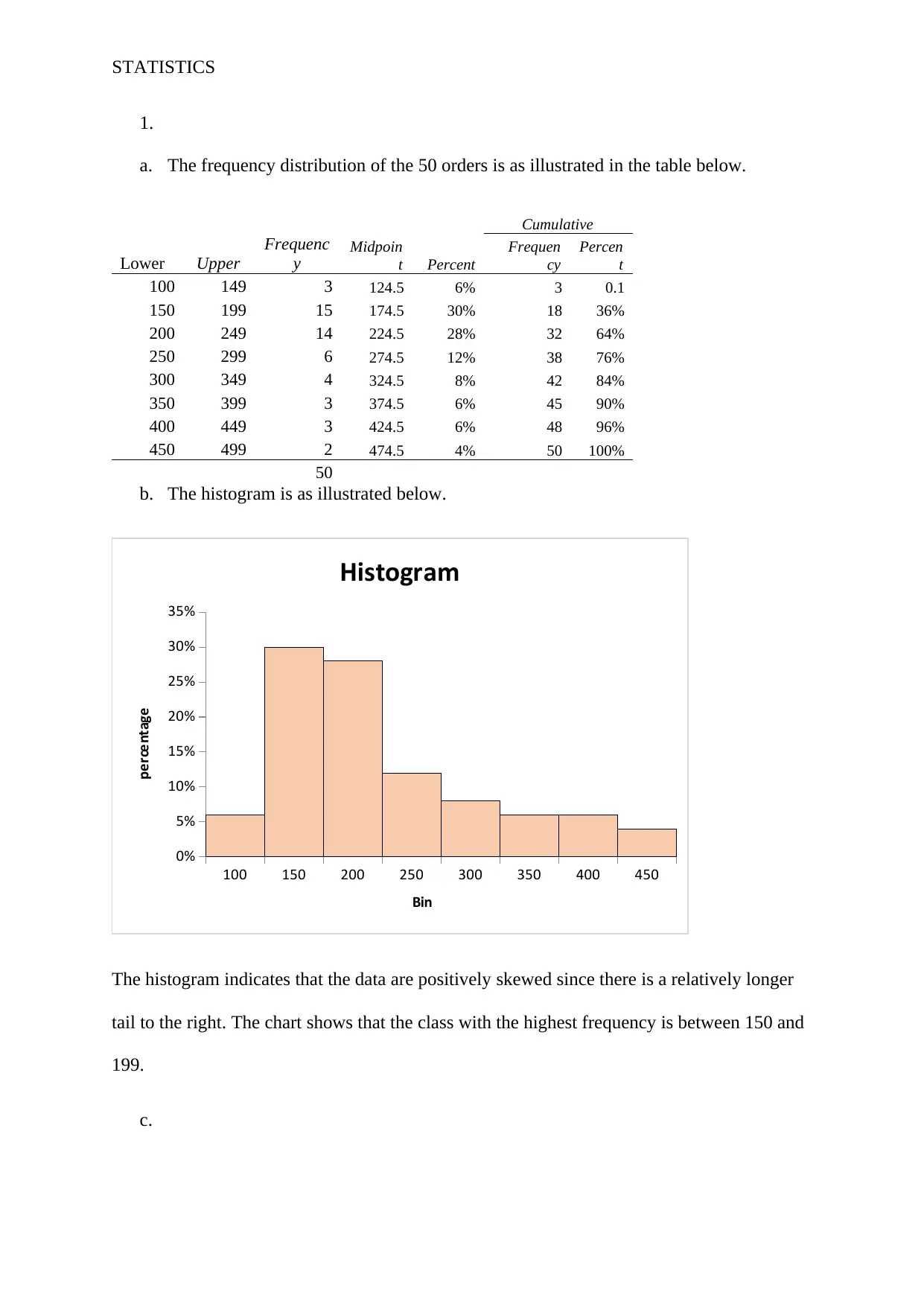
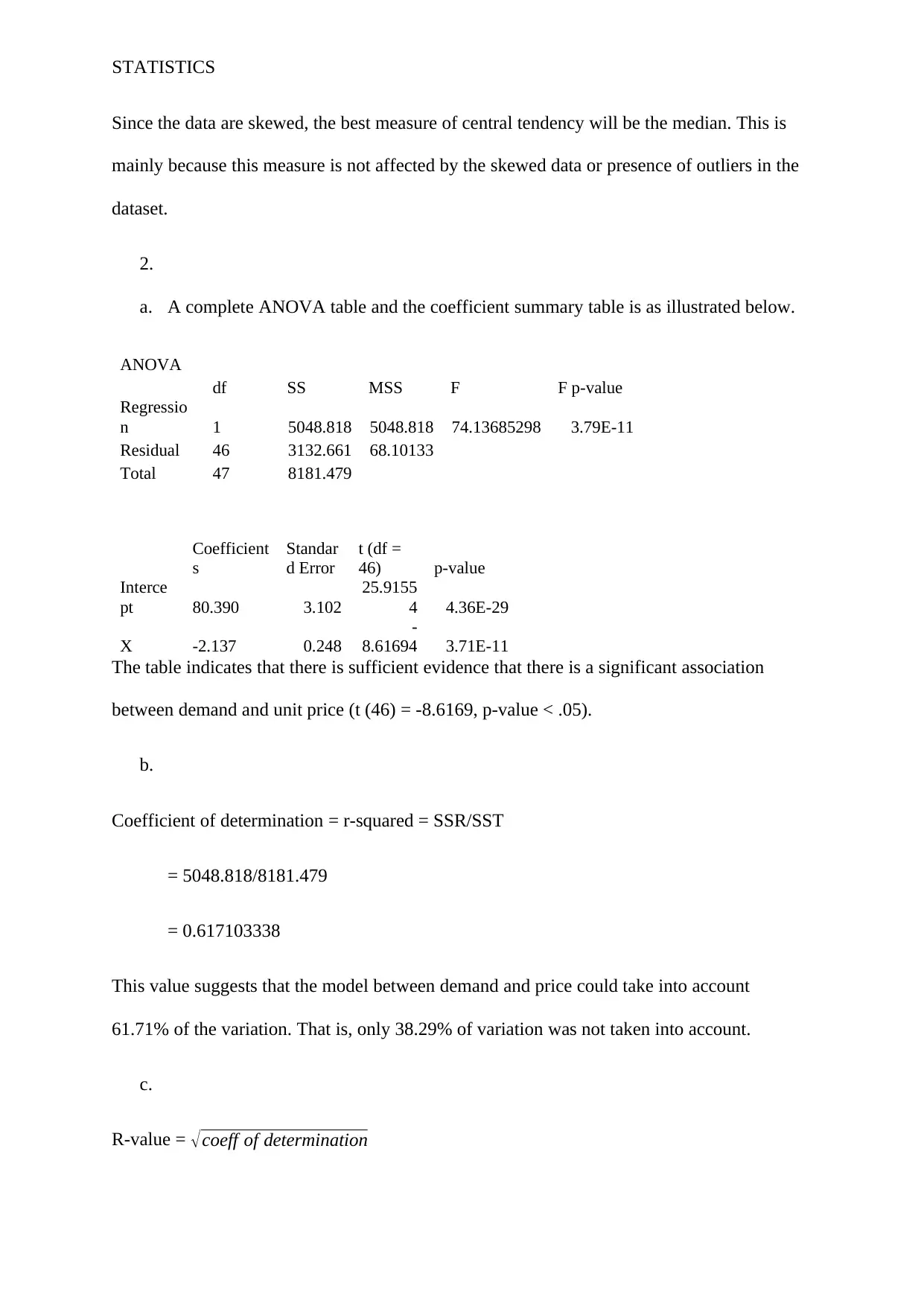
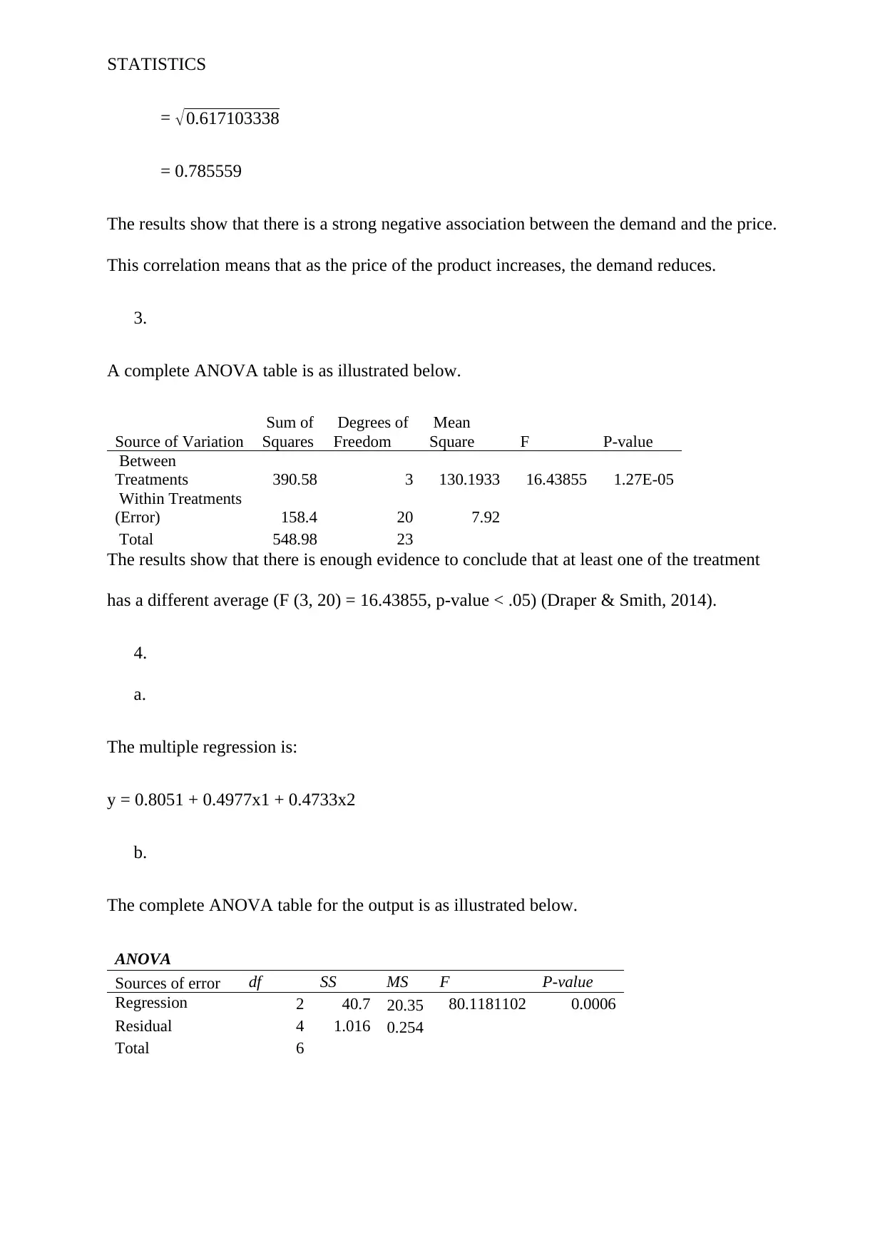
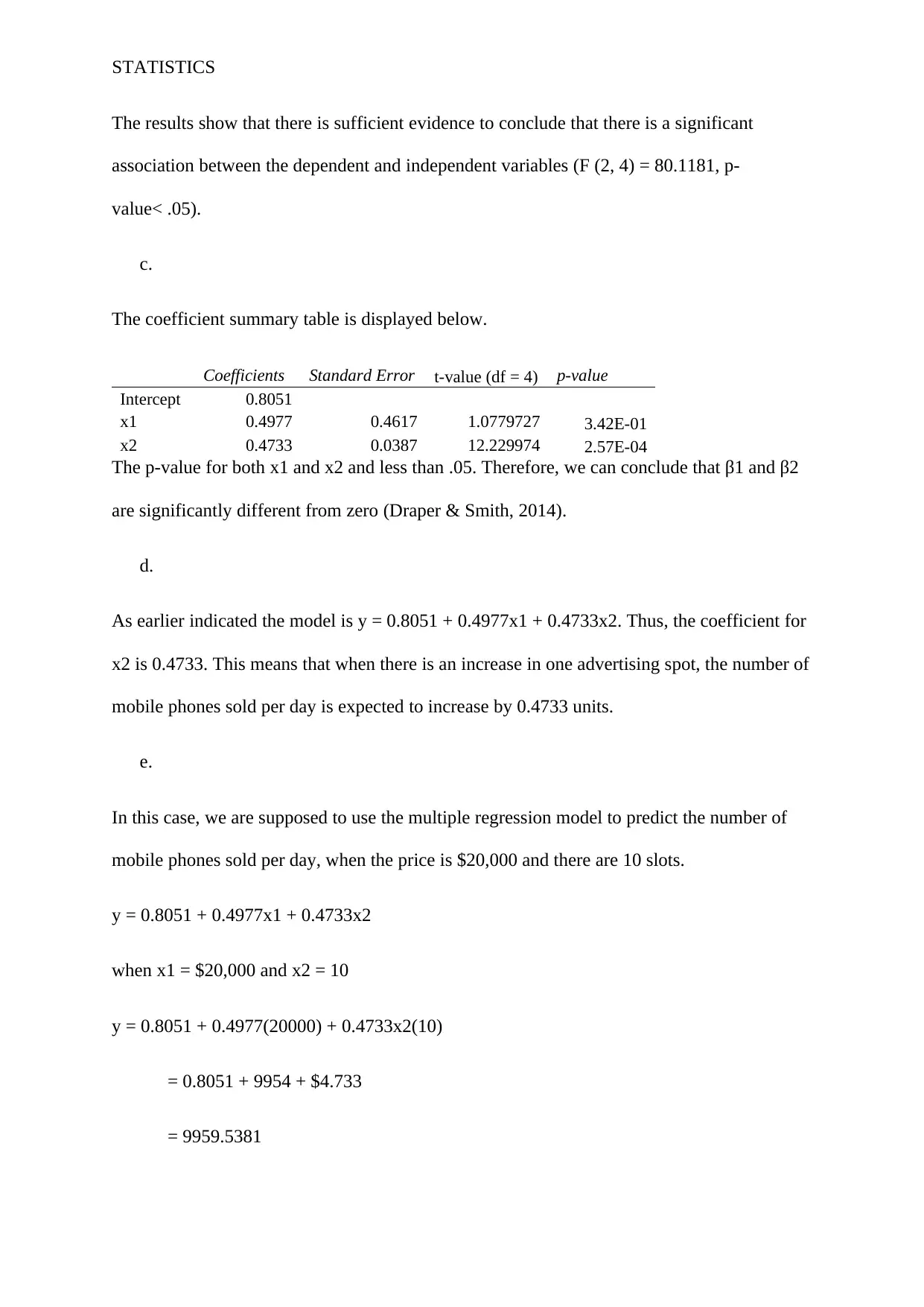
This assignment solution demonstrates statistical analysis techniques, including creating a frequency distribution from order data, interpreting a histogram, and determining the appropriate measure of central tendency for skewed data. It also includes the construction and interpretation of ANOVA tables to assess the significance of relationships between variables, such as demand and unit price. Furthermore, the assignment covers multiple regression analysis, providing a model to predict outcomes based on multiple independent variables and interpreting the coefficients. The solution calculates and interprets R-squared values and p-values to draw conclusions about the statistical significance of the findings. This document is available on Desklib, a platform offering a wealth of student resources.

Running head: STATISTICS
Statistics
Name:
Institution:

STATISTICS
1.
a. The frequency distribution of the 50 orders is as illustrated in the table below.
Cumulative
Lower Upper
Frequenc
y
Midpoin
t Percent
Frequen
cy
Percen
t
100 149 3 124.5 6% 3 0.1
150 199 15 174.5 30% 18 36%
200 249 14 224.5 28% 32 64%
250 299 6 274.5 12% 38 76%
300 349 4 324.5 8% 42 84%
350 399 3 374.5 6% 45 90%
400 449 3 424.5 6% 48 96%
450 499 2 474.5 4% 50 100%
50
b. The histogram is as illustrated below.
100 150 200 250 300 350 400 450
0%
5%
10%
15%
20%
25%
30%
35%
Histogram
Bin
percentage
The histogram indicates that the data are positively skewed since there is a relatively longer
tail to the right. The chart shows that the class with the highest frequency is between 150 and
199.
c.

STATISTICS
Since the data are skewed, the best measure of central tendency will be the median. This is
mainly because this measure is not affected by the skewed data or presence of outliers in the
dataset.
2.
a. A complete ANOVA table and the coefficient summary table is as illustrated below.
ANOVA
df SS MSS F F p-value
Regressio
n 1 5048.818 5048.818 74.13685298 3.79E-11
Residual 46 3132.661 68.10133
Total 47 8181.479
Coefficient
s
Standar
d Error
t (df =
46) p-value
Interce
pt 80.390 3.102
25.9155
4 4.36E-29
X -2.137 0.248
-
8.61694 3.71E-11
The table indicates that there is sufficient evidence that there is a significant association
between demand and unit price (t (46) = -8.6169, p-value < .05).
b.
Coefficient of determination = r-squared = SSR/SST
= 5048.818/8181.479
= 0.617103338
This value suggests that the model between demand and price could take into account
61.71% of the variation. That is, only 38.29% of variation was not taken into account.
c.
R-value = √coeff of determination

STATISTICS
= √0.617103338
= 0.785559
The results show that there is a strong negative association between the demand and the price.
This correlation means that as the price of the product increases, the demand reduces.
3.
A complete ANOVA table is as illustrated below.
Source of Variation
Sum of
Squares
Degrees of
Freedom
Mean
Square F P-value
Between
Treatments 390.58 3 130.1933 16.43855 1.27E-05
Within Treatments
(Error) 158.4 20 7.92
Total 548.98 23
The results show that there is enough evidence to conclude that at least one of the treatment
has a different average (F (3, 20) = 16.43855, p-value < .05) (Draper & Smith, 2014).
4.
a.
The multiple regression is:
y = 0.8051 + 0.4977x1 + 0.4733x2
b.
The complete ANOVA table for the output is as illustrated below.
ANOVA
Sources of error df SS MS F P-value
Regression 2 40.7 20.35 80.1181102 0.0006
Residual 4 1.016 0.254
Total 6

STATISTICS
The results show that there is sufficient evidence to conclude that there is a significant
association between the dependent and independent variables (F (2, 4) = 80.1181, p-
value< .05).
c.
The coefficient summary table is displayed below.
Coefficients Standard Error t-value (df = 4) p-value
Intercept 0.8051
x1 0.4977 0.4617 1.0779727 3.42E-01
x2 0.4733 0.0387 12.229974 2.57E-04
The p-value for both x1 and x2 and less than .05. Therefore, we can conclude that β1 and β2
are significantly different from zero (Draper & Smith, 2014).
d.
As earlier indicated the model is y = 0.8051 + 0.4977x1 + 0.4733x2. Thus, the coefficient for
x2 is 0.4733. This means that when there is an increase in one advertising spot, the number of
mobile phones sold per day is expected to increase by 0.4733 units.
e.
In this case, we are supposed to use the multiple regression model to predict the number of
mobile phones sold per day, when the price is $20,000 and there are 10 slots.
y = 0.8051 + 0.4977x1 + 0.4733x2
when x1 = $20,000 and x2 = 10
y = 0.8051 + 0.4977(20000) + 0.4733x2(10)
= 0.8051 + 9954 + $4.733
= 9959.5381

STATISTICS
This means that approximately 9959.5381 mobile phones will be sold per day.

STATISTICS
References
Draper, N. R., & Smith, H. (2014). Applied regression analysis (Vol. 326). John Wiley &
Sons.