Statistics for Management: Analyzing Earnings, Surveys, and Data
VerifiedAdded on 2023/01/11
|18
|1332
|93
Homework Assignment
AI Summary
This statistics assignment analyzes earnings data in both public and private sectors, comparing men's and women's earnings using t-tests to determine statistical significance. It also examines a survey of leisure center staff earnings, calculating median, quartiles, mean, and standard deviation. The assignment includes comparisons of data between Manchester and London, along with an analysis of economic order quantity (EOQ) for olive oil deliveries and a linear regression model to explore the relationship between the number of bedrooms and house prices in different streets. The document provides detailed calculations and interpretations of the statistical results, offering a comprehensive understanding of the concepts covered.

Statistics for Management
Paraphrase This Document
Need a fresh take? Get an instant paraphrase of this document with our AI Paraphraser

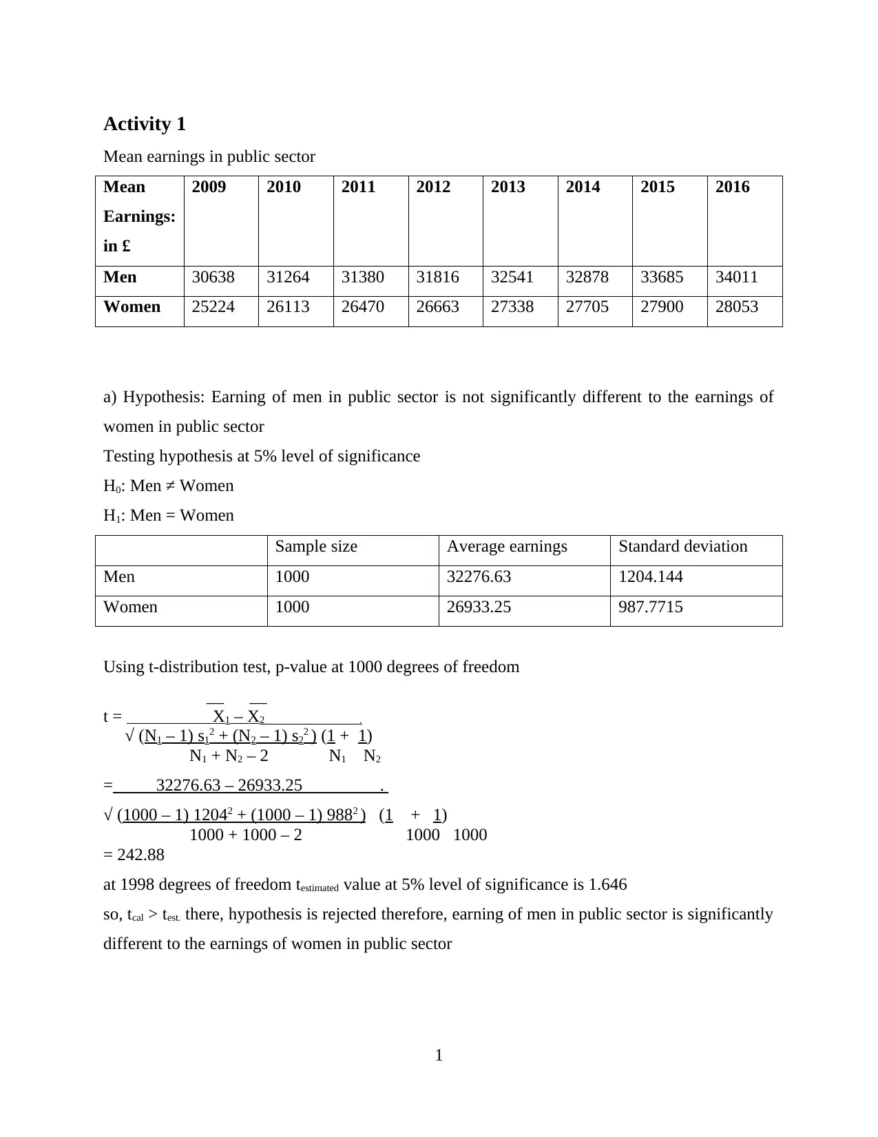
Activity 1
Mean earnings in public sector
Mean
Earnings:
in £
2009 2010 2011 2012 2013 2014 2015 2016
Men 30638 31264 31380 31816 32541 32878 33685 34011
Women 25224 26113 26470 26663 27338 27705 27900 28053
a) Hypothesis: Earning of men in public sector is not significantly different to the earnings of
women in public sector
Testing hypothesis at 5% level of significance
H0: Men ≠ Women
H1: Men = Women
Sample size Average earnings Standard deviation
Men 1000 32276.63 1204.144
Women 1000 26933.25 987.7715
Using t-distribution test, p-value at 1000 degrees of freedom
__ __
t = X1 – X2 .
√ (N1 – 1) s12 + (N2 – 1) s22 ) (1 + 1)
N1 + N2 – 2 N1 N2
= 32276.63 – 26933.25 .
√ (1000 – 1) 12042 + (1000 – 1) 9882 ) (1 + 1)
1000 + 1000 – 2 1000 1000
= 242.88
at 1998 degrees of freedom testimated value at 5% level of significance is 1.646
so, tcal > test. there, hypothesis is rejected therefore, earning of men in public sector is significantly
different to the earnings of women in public sector
1
⊘ This is a preview!⊘
Do you want full access?
Subscribe today to unlock all pages.

Trusted by 1+ million students worldwide
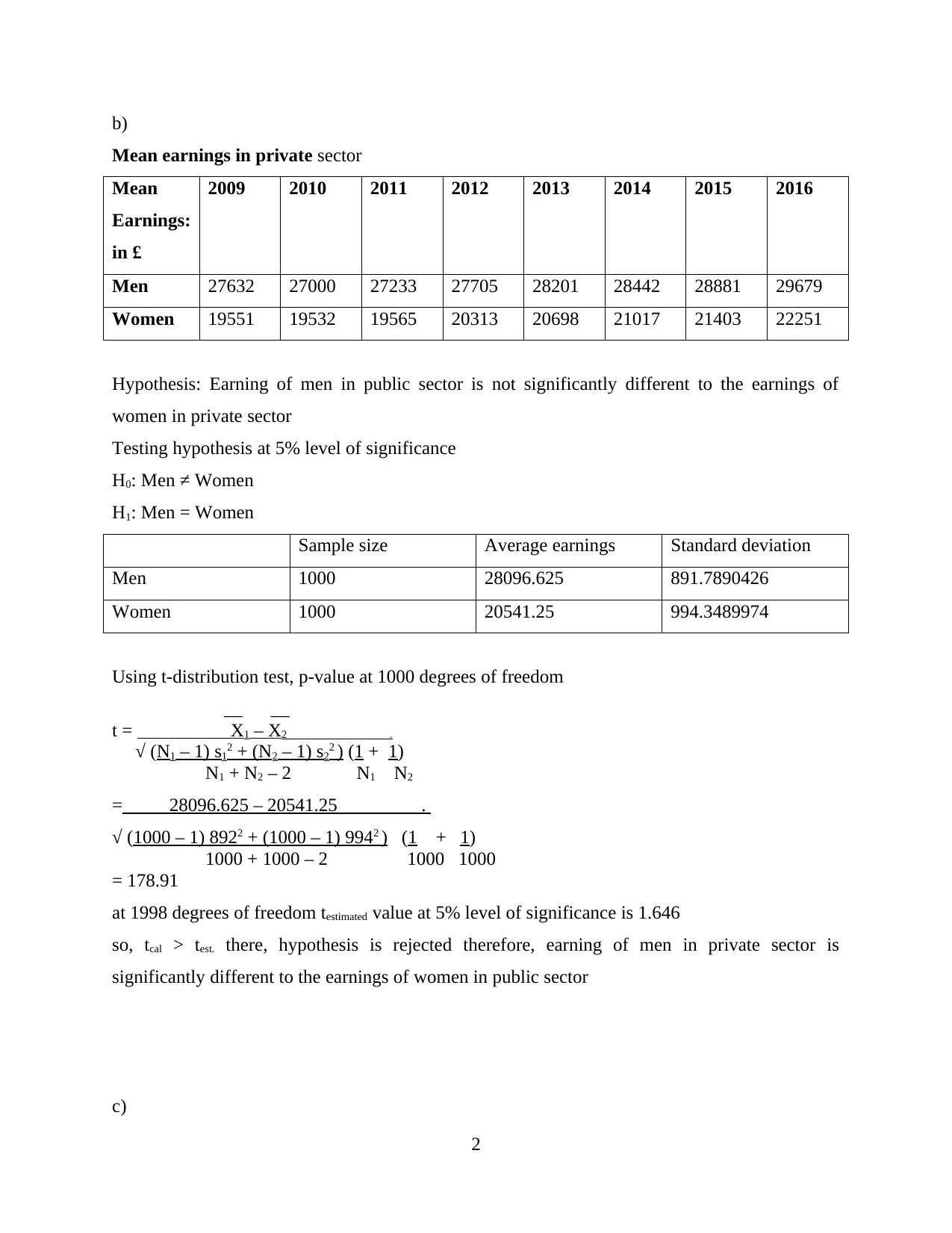
b)
Mean earnings in private sector
Mean
Earnings:
in £
2009 2010 2011 2012 2013 2014 2015 2016
Men 27632 27000 27233 27705 28201 28442 28881 29679
Women 19551 19532 19565 20313 20698 21017 21403 22251
Hypothesis: Earning of men in public sector is not significantly different to the earnings of
women in private sector
Testing hypothesis at 5% level of significance
H0: Men ≠ Women
H1: Men = Women
Sample size Average earnings Standard deviation
Men 1000 28096.625 891.7890426
Women 1000 20541.25 994.3489974
Using t-distribution test, p-value at 1000 degrees of freedom
__ __
t = X1 – X2 .
√ (N1 – 1) s12 + (N2 – 1) s22 ) (1 + 1)
N1 + N2 – 2 N1 N2
= 28096.625 – 20541.25 .
√ (1000 – 1) 8922 + (1000 – 1) 9942 ) (1 + 1)
1000 + 1000 – 2 1000 1000
= 178.91
at 1998 degrees of freedom testimated value at 5% level of significance is 1.646
so, tcal > test. there, hypothesis is rejected therefore, earning of men in private sector is
significantly different to the earnings of women in public sector
c)
2
Paraphrase This Document
Need a fresh take? Get an instant paraphrase of this document with our AI Paraphraser
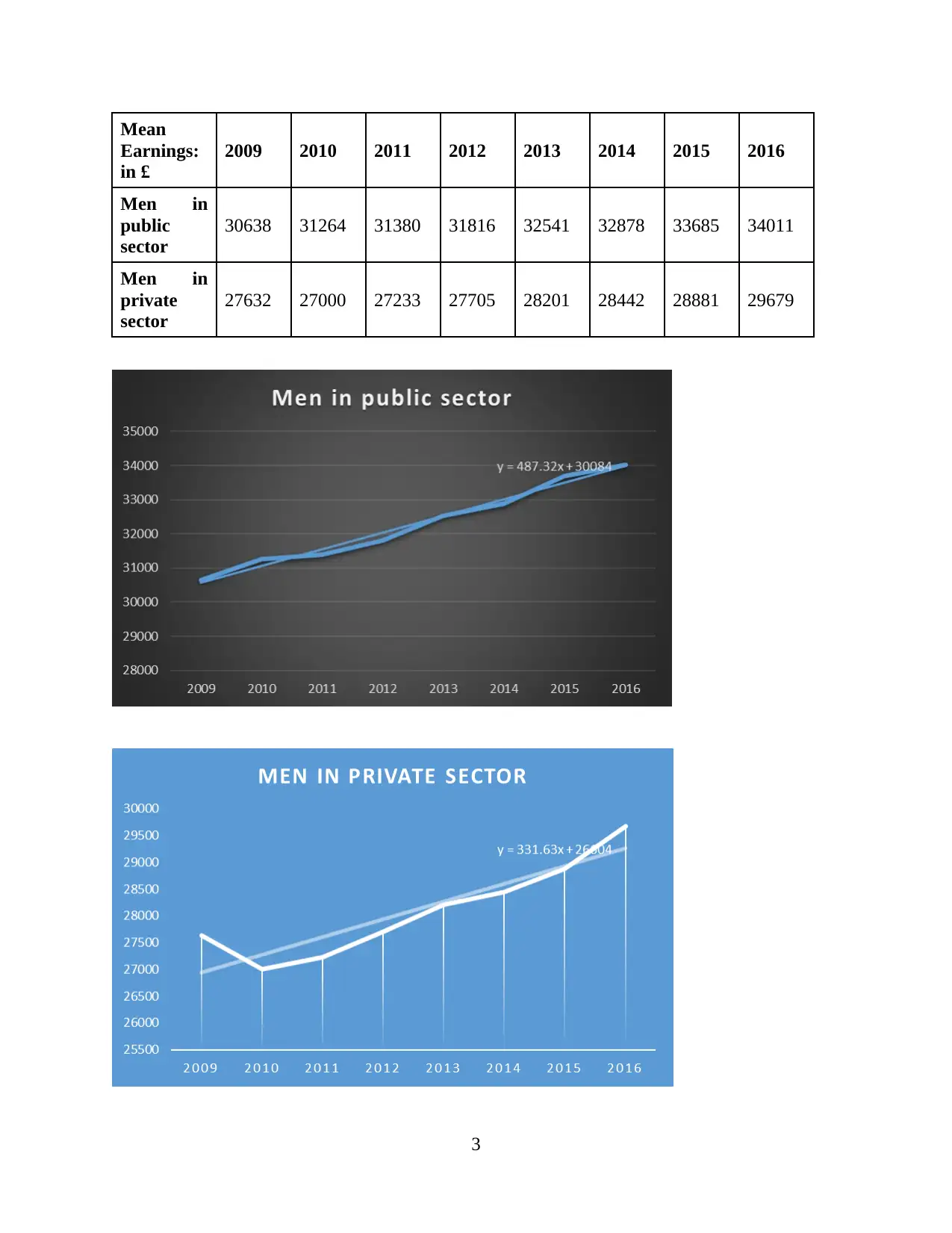
Mean
Earnings:
in £
2009 2010 2011 2012 2013 2014 2015 2016
Men in
public
sector
30638 31264 31380 31816 32541 32878 33685 34011
Men in
private
sector
27632 27000 27233 27705 28201 28442 28881 29679
3
Earnings:
in £
2009 2010 2011 2012 2013 2014 2015 2016
Men in
public
sector
30638 31264 31380 31816 32541 32878 33685 34011
Men in
private
sector
27632 27000 27233 27705 28201 28442 28881 29679
3
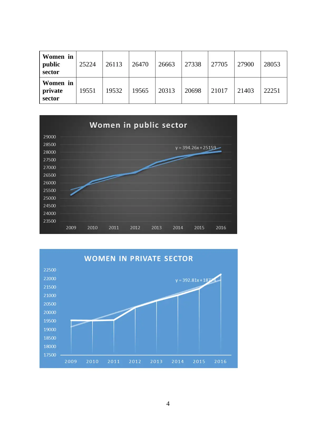
Women in
public
sector
25224 26113 26470 26663 27338 27705 27900 28053
Women in
private
sector
19551 19532 19565 20313 20698 21017 21403 22251
4
public
sector
25224 26113 26470 26663 27338 27705 27900 28053
Women in
private
sector
19551 19532 19565 20313 20698 21017 21403 22251
4
⊘ This is a preview!⊘
Do you want full access?
Subscribe today to unlock all pages.

Trusted by 1+ million students worldwide
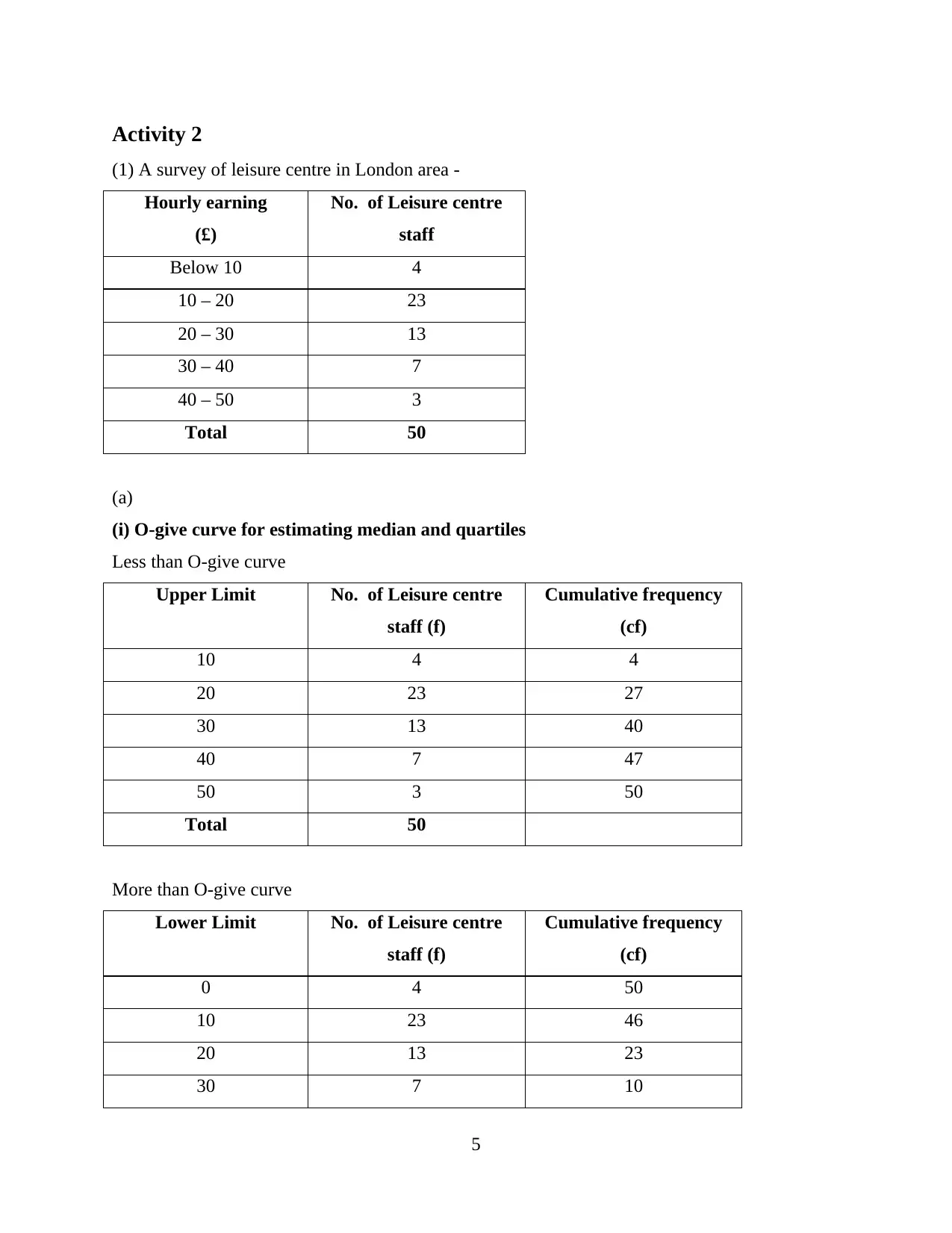
Activity 2
(1) A survey of leisure centre in London area -
Hourly earning
(£)
No. of Leisure centre
staff
Below 10 4
10 – 20 23
20 – 30 13
30 – 40 7
40 – 50 3
Total 50
(a)
(i) O-give curve for estimating median and quartiles
Less than O-give curve
Upper Limit No. of Leisure centre
staff (f)
Cumulative frequency
(cf)
10 4 4
20 23 27
30 13 40
40 7 47
50 3 50
Total 50
More than O-give curve
Lower Limit No. of Leisure centre
staff (f)
Cumulative frequency
(cf)
0 4 50
10 23 46
20 13 23
30 7 10
5
Paraphrase This Document
Need a fresh take? Get an instant paraphrase of this document with our AI Paraphraser
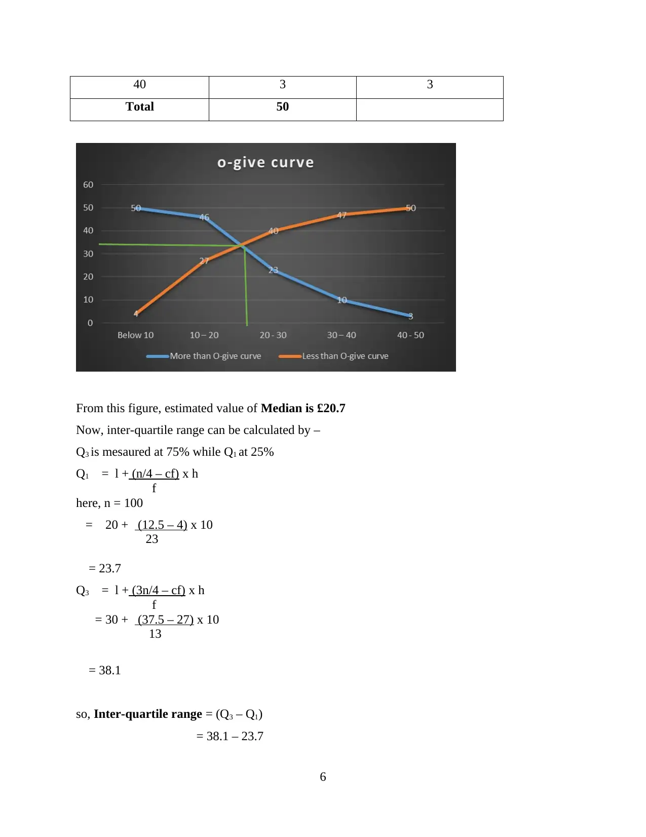
40 3 3
Total 50
From this figure, estimated value of Median is £20.7
Now, inter-quartile range can be calculated by –
Q3 is mesaured at 75% while Q1 at 25%
Q1 = l + (n/4 – cf) x h
f
here, n = 100
= 20 + (12.5 – 4) x 10
23
= 23.7
Q3 = l + (3n/4 – cf) x h
f
= 30 + (37.5 – 27) x 10
13
= 38.1
so, Inter-quartile range = (Q3 – Q1)
= 38.1 – 23.7
6
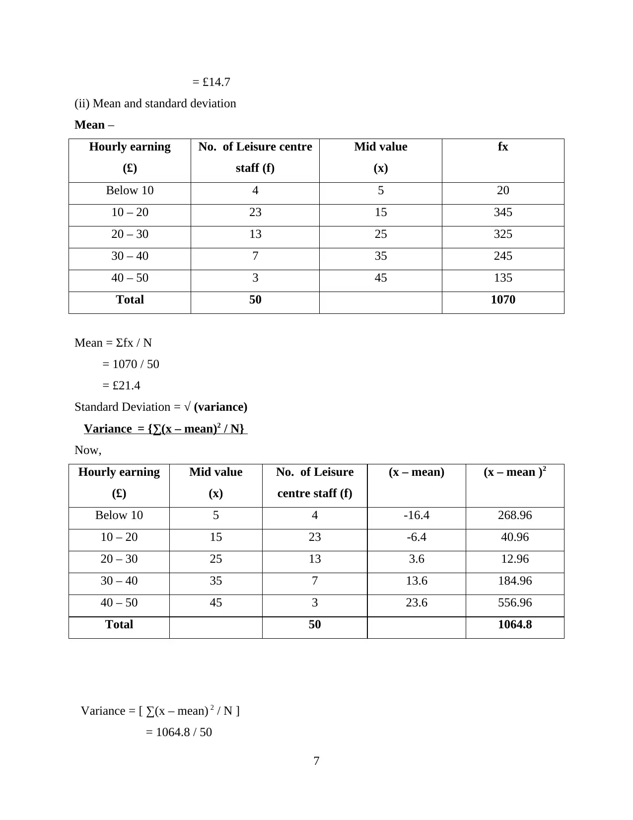
= £14.7
(ii) Mean and standard deviation
Mean –
Hourly earning
(£)
No. of Leisure centre
staff (f)
Mid value
(x)
fx
Below 10 4 5 20
10 – 20 23 15 345
20 – 30 13 25 325
30 – 40 7 35 245
40 – 50 3 45 135
Total 50 1070
Mean = Σfx / N
= 1070 / 50
= £21.4
Standard Deviation = √ (variance)
Variance = {∑(x – mean)2 / N}
Now,
Hourly earning
(£)
Mid value
(x)
No. of Leisure
centre staff (f)
(x – mean) (x – mean )2
Below 10 5 4 -16.4 268.96
10 – 20 15 23 -6.4 40.96
20 – 30 25 13 3.6 12.96
30 – 40 35 7 13.6 184.96
40 – 50 45 3 23.6 556.96
Total 50 1064.8
Variance = [ ∑(x – mean) 2 / N ]
= 1064.8 / 50
7
⊘ This is a preview!⊘
Do you want full access?
Subscribe today to unlock all pages.

Trusted by 1+ million students worldwide
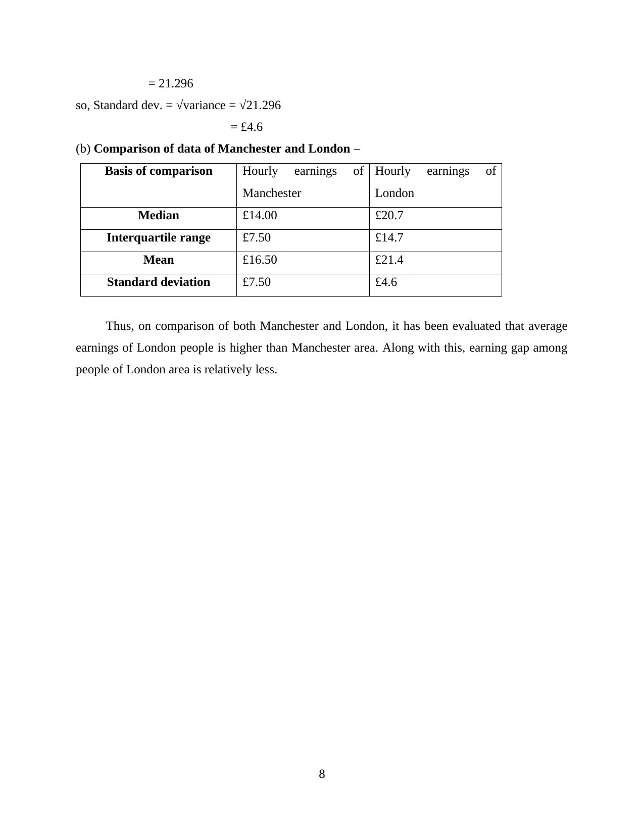
= 21.296
so, Standard dev. = √variance = √21.296
= £4.6
(b) Comparison of data of Manchester and London –
Basis of comparison Hourly earnings of
Manchester
Hourly earnings of
London
Median £14.00 £20.7
Interquartile range £7.50 £14.7
Mean £16.50 £21.4
Standard deviation £7.50 £4.6
Thus, on comparison of both Manchester and London, it has been evaluated that average
earnings of London people is higher than Manchester area. Along with this, earning gap among
people of London area is relatively less.
8
Paraphrase This Document
Need a fresh take? Get an instant paraphrase of this document with our AI Paraphraser
Question 3:
(a)
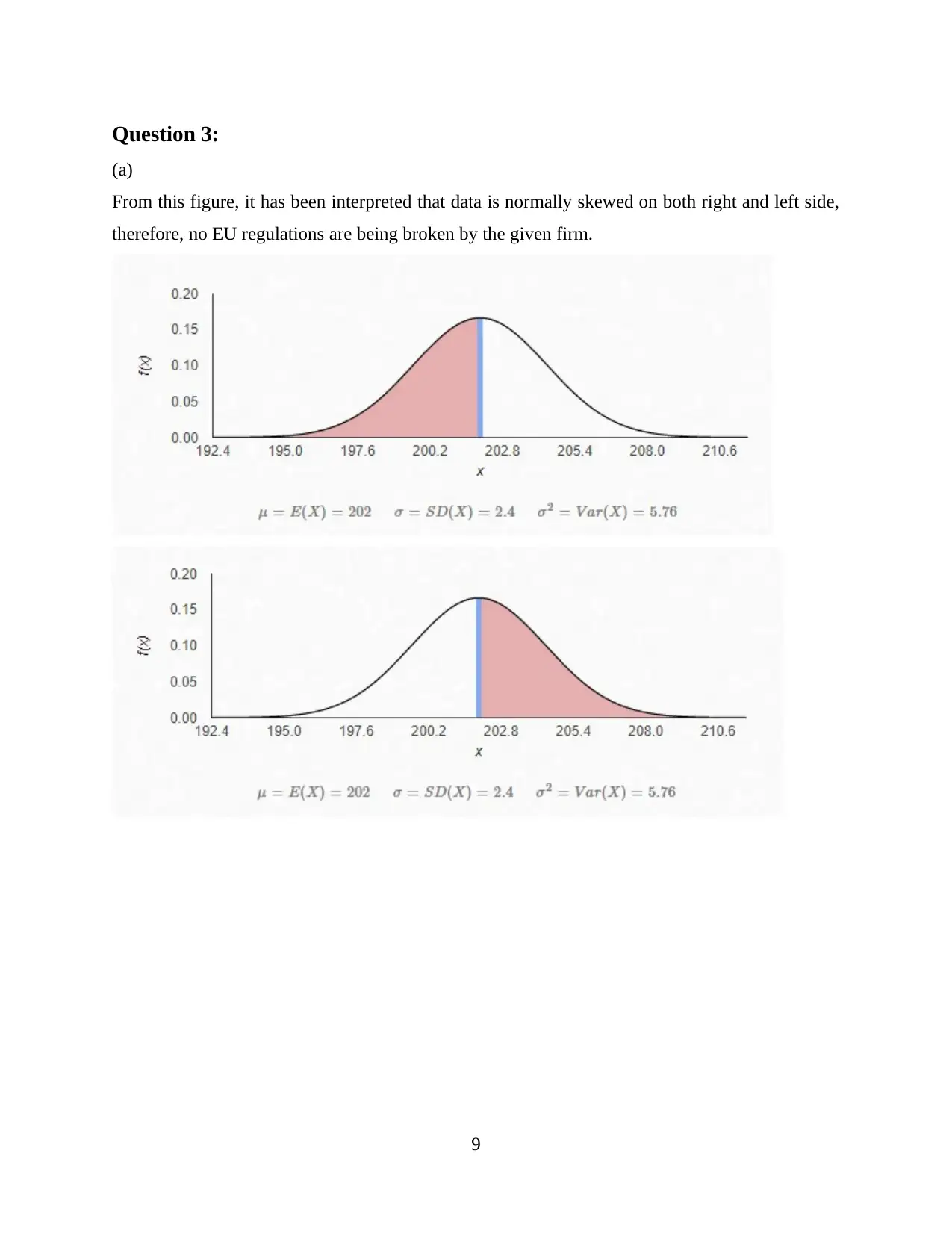
From this figure, it has been interpreted that data is normally skewed on both right and left side,
therefore, no EU regulations are being broken by the given firm.
9
(a)
From this figure, it has been interpreted that data is normally skewed on both right and left side,
therefore, no EU regulations are being broken by the given firm.
9
b)
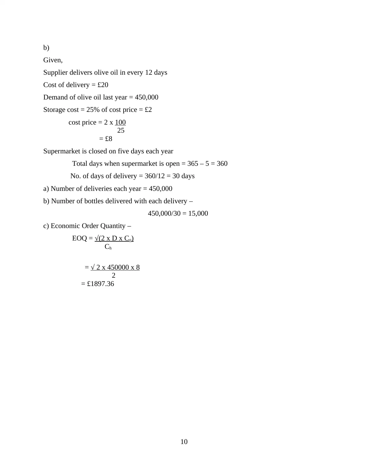
Given,
Supplier delivers olive oil in every 12 days
Cost of delivery = £20
Demand of olive oil last year = 450,000
Storage cost = 25% of cost price = £2
cost price = 2 x 100
25
= £8
Supermarket is closed on five days each year
Total days when supermarket is open = 365 – 5 = 360
No. of days of delivery = 360/12 = 30 days
a) Number of deliveries each year = 450,000
b) Number of bottles delivered with each delivery –
450,000/30 = 15,000
c) Economic Order Quantity –
EOQ = √(2 x D x Co)
Ch
= √ 2 x 450000 x 8
2
= £1897.36
10
⊘ This is a preview!⊘
Do you want full access?
Subscribe today to unlock all pages.

Trusted by 1+ million students worldwide
1 out of 18
Related Documents
Your All-in-One AI-Powered Toolkit for Academic Success.
+13062052269
info@desklib.com
Available 24*7 on WhatsApp / Email
![[object Object]](/_next/static/media/star-bottom.7253800d.svg)
Unlock your academic potential
Copyright © 2020–2026 A2Z Services. All Rights Reserved. Developed and managed by ZUCOL.


