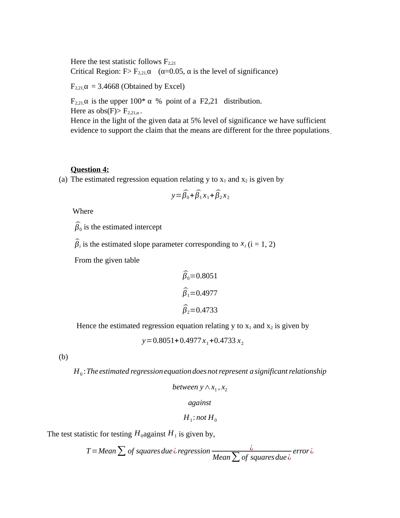
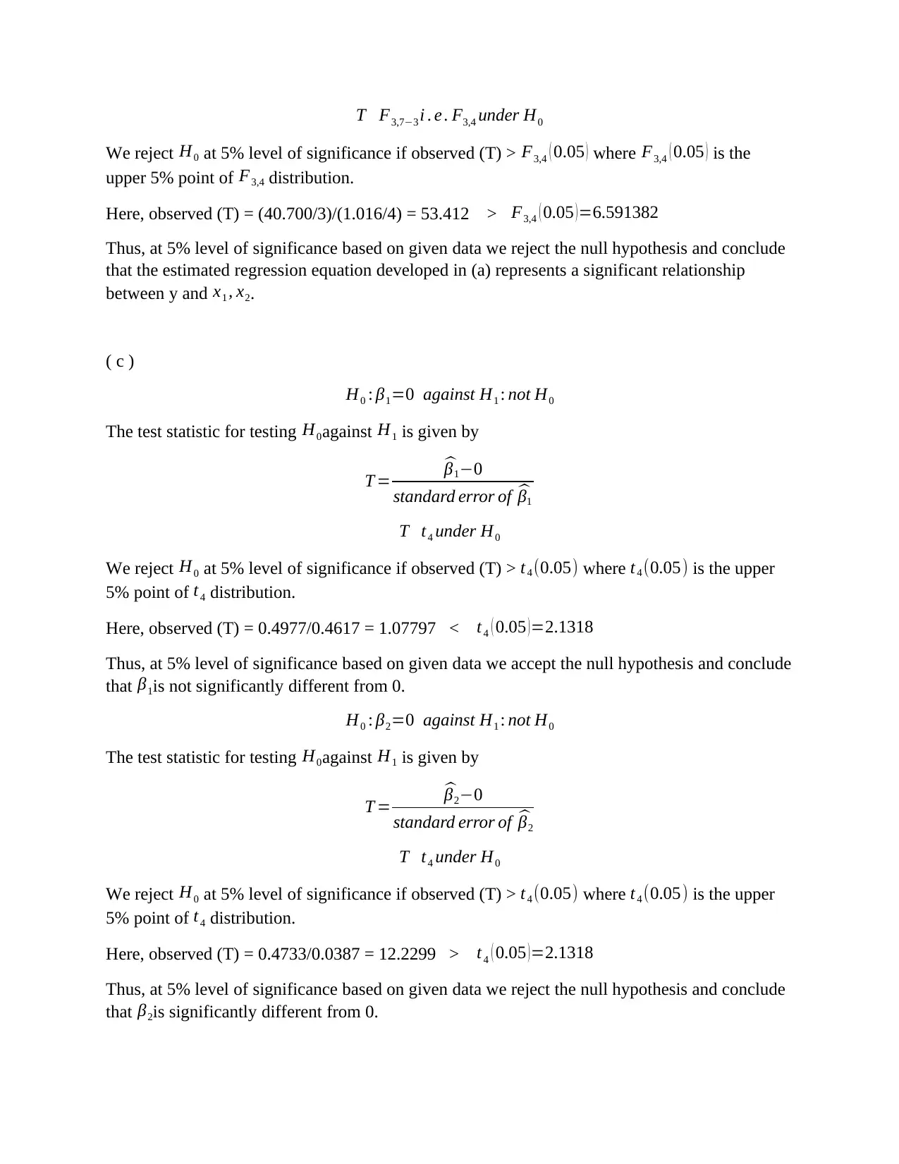
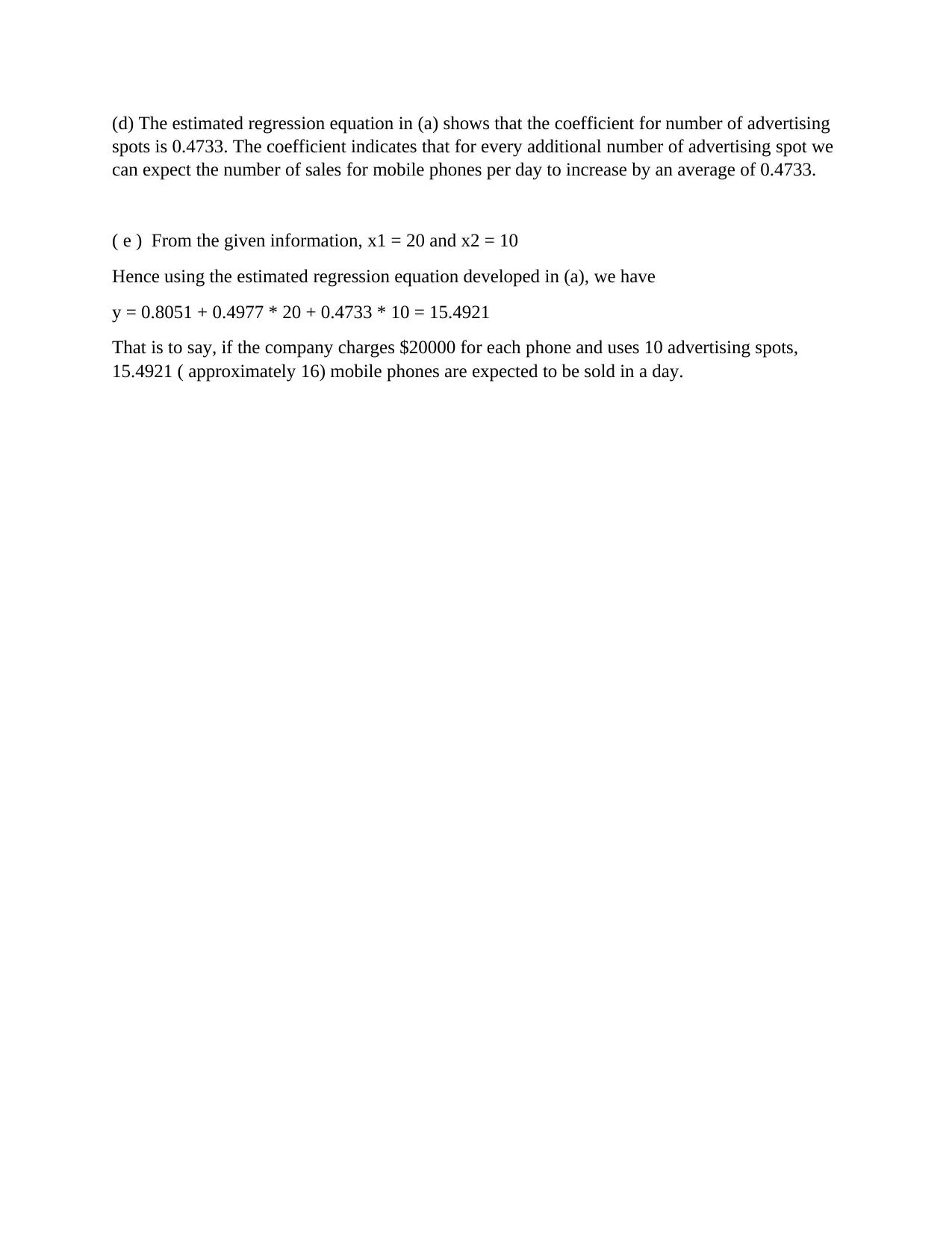
Statistics Homework Assignment: Data Analysis and Regression

This statistics homework assignment provides a comprehensive analysis of data using various statistical methods. The assignment begins with the calculation of range and the creation of frequency, relative frequency, and percentage frequency distributions for a given dataset, along with a visual representation through a histogram. The analysis then moves on to regression analysis, examining the relationship between demand and unit price, including the calculation of the coefficient of variation and correlation coefficient. Furthermore, the assignment investigates the comparison of means across three populations using ANOVA. Finally, the assignment concludes with a multiple regression analysis, exploring the relationship between sales and advertising spots and price, along with interpretations of coefficients and predictions based on the regression equation. The assignment provides detailed calculations and interpretations, offering a clear understanding of the statistical concepts and their application.

Question 1:
a) From the data using excel we find out that, Minimum=$123 ,Maximum= $490 i.e.
Range=$490-$123=$367.
We have a dataset of 50 observations. We have to make frequency distribution, relative
frequency distribution, percentage frequency distribution with class width of $50
Next, we divide the data range into 5 parts.
Frequency Distribution:
Furniture portion of each order(in dollars) Frequency
120-170 8
170-220 15
220-270 12
270-320 4
320-370 5
370-420 2
420-470 2
470-520 2
Table 1:Frequency Distribution showing furniture portion of the 50 orders
Relative Frequency Distribution:
Furniture portion of each order(in dollars) Relative Frequency
120-170 0.16
170-220 0.3
220-270 0.24
270-320 0.08
320-370 0.1
370-420 0.04
420-470 0.04
470-520 0.04
Table 2: Relative Frequency Distribution showing furniture portion of the 50 orders

Percentage frequency Distribution:
Furniture portion of each order(in dollars) Percentage Frequency
120-170 16
170-220 30
220-270 24
270-320 8
320-370 10
370-420 4
420-470 4
470-520 4
Table 3: Percentage Frequency Distribution showing furniture portion of the 50 orders
b)
Furniture portion of each order(in dollars) Percentage Frequency
120-170 16
170-220 30
220-270 24
270-320 8
320-370 10
370-420 4
420-470 4
470-520 4
From the above percentage Frequency table we get the following Histogram by using
Excel:

120-170 170-220 220-270 270-320 320-370 370-420 420-470 470-520
0
5
10
15
20
25
30
35
Percentage frequency Histogram showing
furniture portion
Diagram 1: Percentage Frequency Histogram Showing Furniture portion of Orders
From the percentage frequency histogram we get that the furniture portion of each order
follows a positively skewed distribution i.e. a right skewed distribution.
c)
As the data is a skewed data, so median would be a good measure of location for this
dataset.
Question 2:
a)
The Regression output shows the anova table of relating to the variables Y(demand),
X(Price).
H0 :The estimated regression equation does not represent a significant relationship
between Y ∧X
against
H1 : not H0
Here Y(demand) is the response variable and X(Price) is the independent variable.
Here SSR=5048.818 (SSR=Sum of Squares due to Regression) and SSRes =3132.661
( SSRes = Sum of Squares due to Residuals)
Here degrees of freedom for the SSR part is 1 and for SSRes part Df=46 .

Now, the value of the F statistic=
SSR
1
SSRes
46
=74.13685298
Here we conclude that the regression is significant as the value of the test statistic is
greater than critical value F1,46,α =4.051749 (α=0.05, α is the level of significance)
Hence in the light of the given data at 5% level of significance we have sufficient
evidence to support the claim that the demand and unit price are related.
.
b)
Coefficient of Variation=∑ of squares due ¿ Regression ¿
Total ∑ of Squares = 5048.818
8181.479
=0.617103337
Hence, 61.71 % of the variation in demand(Y) is explained by the unit price(X) by the
regression equation.
c)
Here the correlation coefficient= √Coefficient of Variation =R =0.78555925
Hence there is a strong positive correlation between the independent
variable(x: unit price),dependent variable (Y: demand) .
Question 3:
We are interested whether there is a significant difference in the means of the three
populations.
Let μ1,μ2 , μ3 denote the population means of three populations.
H0 : μ1=μ2=μ3 vs H1 : Not H0
Note: Here the degrees of freedom for Between treatments=3-1=2
Total degrees of freedom=23 .
Hence Degrees of freedom for within treatments(error) = 23-2=21
Here the test statistic ,
F statistic= ∑ of squares due ¿ treatments
2
¿
SS due ¿ Error
21 ¿=
390.58
2
158.4
21
=25.8907197

Here the test statistic follows F2,21
Critical Region: F> F2,21,α (α=0.05, α is the level of significance)
F2,21,α = 3.4668 (Obtained by Excel)
F2,21,α is the upper 100* α % point of a F2,21 distribution.
Here as obs(F)> F2,21,α .
Hence in the light of the given data at 5% level of significance we have sufficient
evidence to support the claim that the means are different for the three populations..
Question 4:
(a) The estimated regression equation relating y to x1 and x2 is given by
y= ^β0 + ^β1 x1 + ^β2 x2
Where
^β0 is the estimated intercept
^βi is the estimated slope parameter corresponding to xi (i = 1, 2)
From the given table
^β0=0.8051
^β1=0.4977
^β2=0.4733
Hence the estimated regression equation relating y to x1 and x2 is given by
y=0.8051+0.4977 x1 +0.4733 x2
(b)
H0 :The estimated regression equation does not represent a significant relationship
between y ∧x1 , x2
against
H1 : not H0
The test statistic for testing H0against H1 is given by,
T =Mean ∑ of squares due ¿ regression ¿
Mean ∑ of squares due ¿ error ¿

T F3,7−3 i . e . F3,4 under H0
We reject H0 at 5% level of significance if observed (T) > F3,4 ( 0.05 ) where F3,4 ( 0.05 ) is the
upper 5% point of F3,4 distribution.
Here, observed (T) = (40.700/3)/(1.016/4) = 53.412 > F3,4 ( 0.05 )=6.591382
Thus, at 5% level of significance based on given data we reject the null hypothesis and conclude
that the estimated regression equation developed in (a) represents a significant relationship
between y and x1 , x2.
( c )
H0 : β1=0 against H1 : not H0
The test statistic for testing H0against H1 is given by
T =
^β1−0
standard error of ^β1
T t4 under H0
We reject H0 at 5% level of significance if observed (T) > t4 (0.05) where t4 (0.05) is the upper
5% point of t4 distribution.
Here, observed (T) = 0.4977/0.4617 = 1.07797 < t4 ( 0.05 ) =2.1318
Thus, at 5% level of significance based on given data we accept the null hypothesis and conclude
that β1is not significantly different from 0.
H0 : β2=0 against H1 : not H0
The test statistic for testing H0against H1 is given by
T =
^β2−0
standard error of ^β2
T t4 under H0
We reject H0 at 5% level of significance if observed (T) > t4 (0.05) where t4 (0.05) is the upper
5% point of t4 distribution.
Here, observed (T) = 0.4733/0.0387 = 12.2299 > t4 ( 0.05 )=2.1318
Thus, at 5% level of significance based on given data we reject the null hypothesis and conclude
that β2is significantly different from 0.

(d) The estimated regression equation in (a) shows that the coefficient for number of advertising
spots is 0.4733. The coefficient indicates that for every additional number of advertising spot we
can expect the number of sales for mobile phones per day to increase by an average of 0.4733.
( e ) From the given information, x1 = 20 and x2 = 10
Hence using the estimated regression equation developed in (a), we have
y = 0.8051 + 0.4977 * 20 + 0.4733 * 10 = 15.4921
That is to say, if the company charges $20000 for each phone and uses 10 advertising spots,
15.4921 ( approximately 16) mobile phones are expected to be sold in a day.