Statistics Assignment: Financial Data Analysis and Probability

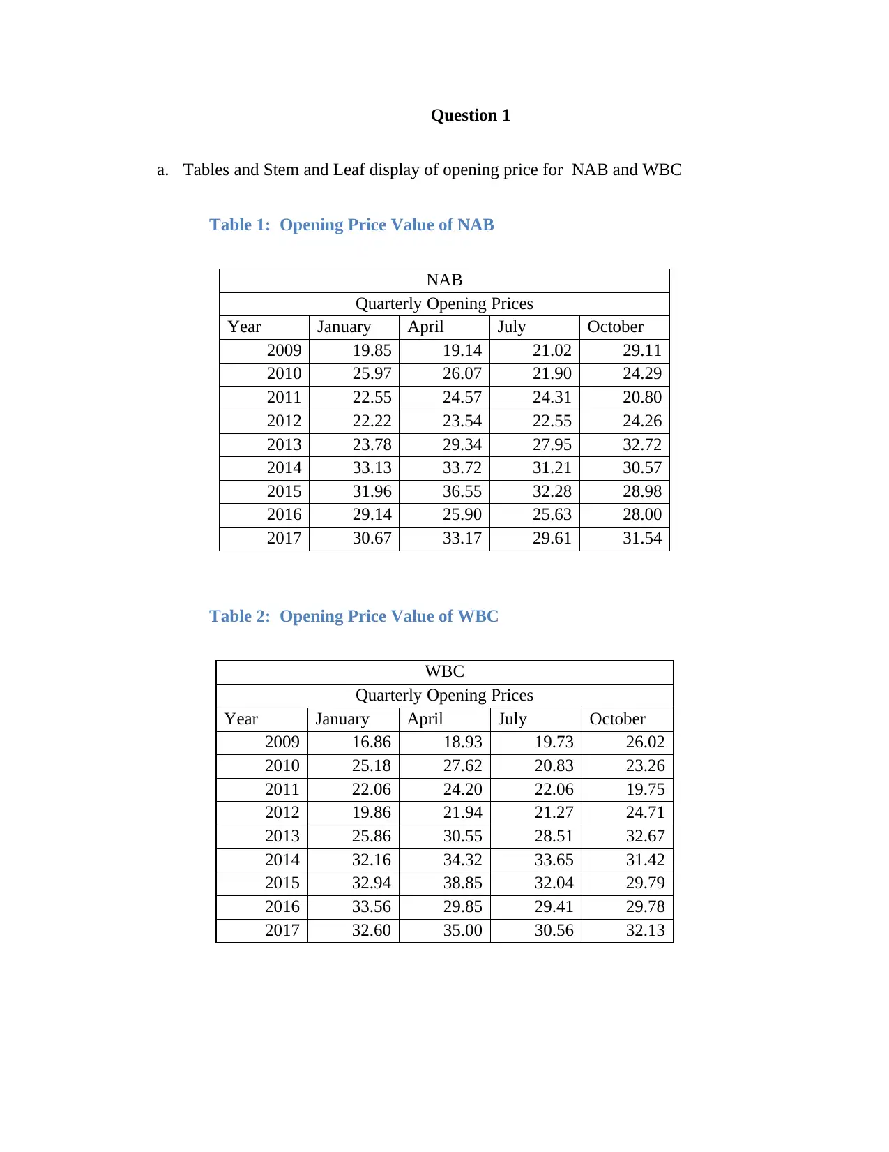
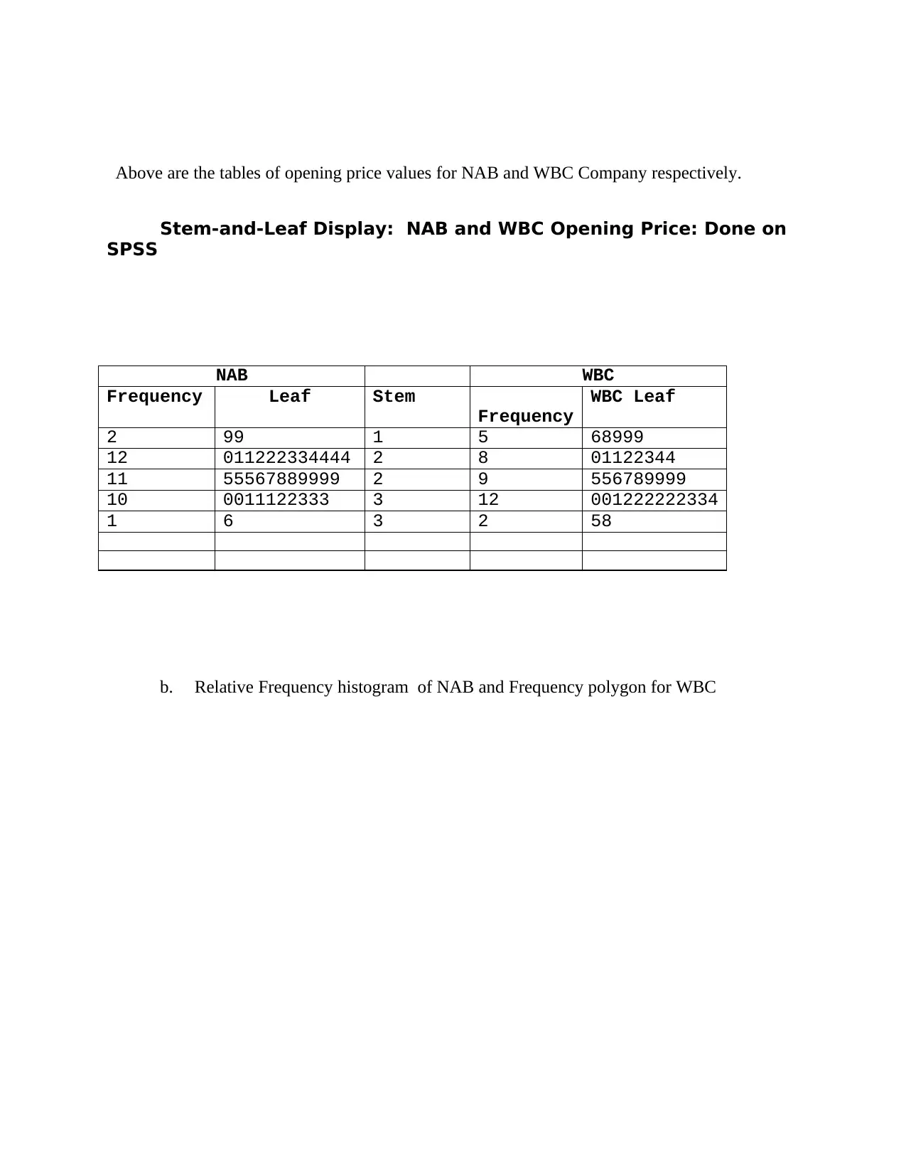
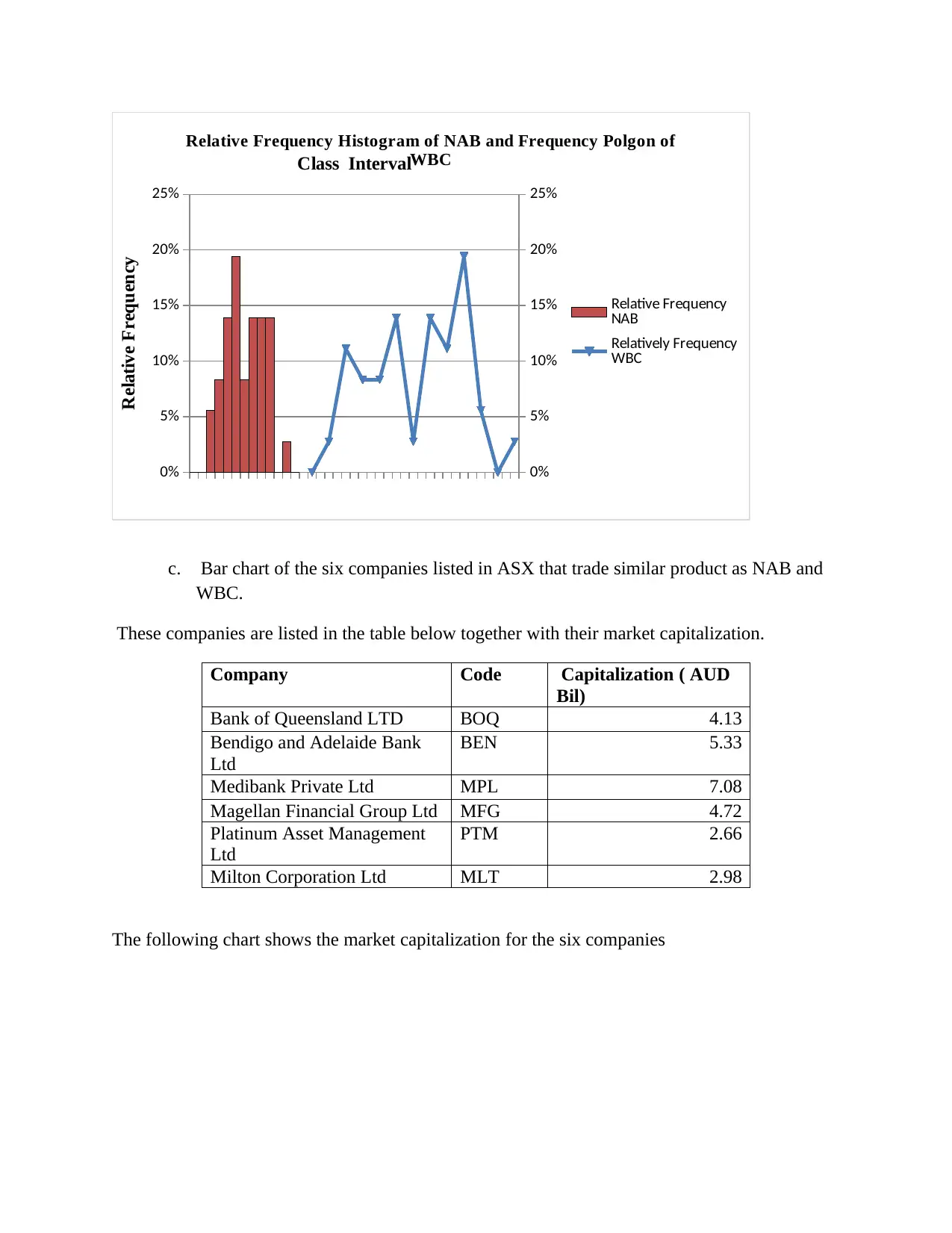
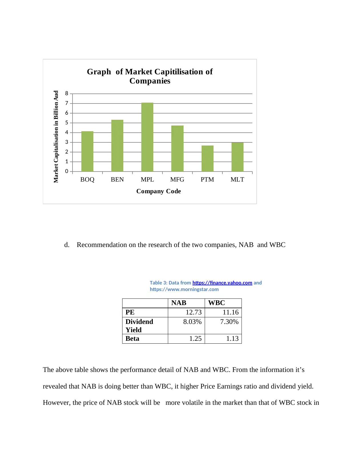
This statistics assignment analyzes financial data, applying various statistical methods to draw conclusions. The assignment includes constructing tables and stem-and-leaf displays of opening prices for NAB and WBC, creating histograms, and bar charts to visualize market capitalization. It explores probability calculations, including conditional probabilities and the application of binomial and normal distributions. Hypothesis testing, confidence intervals, and the use of Excel and SPSS for computations are also demonstrated. The analysis covers topics like the probability of household internet access, the impact of temperature on air, and the probability of sample percentages. The solution provides a comprehensive approach to statistical analysis, covering descriptive statistics, probability, and inferential statistics.

Statistics Assignment
Student’s Name
Institution Affiliation

Question 1
a. Tables and Stem and Leaf display of opening price for NAB and WBC
Table 1: Opening Price Value of NAB
NAB
Quarterly Opening Prices
Year January April July October
2009 19.85 19.14 21.02 29.11
2010 25.97 26.07 21.90 24.29
2011 22.55 24.57 24.31 20.80
2012 22.22 23.54 22.55 24.26
2013 23.78 29.34 27.95 32.72
2014 33.13 33.72 31.21 30.57
2015 31.96 36.55 32.28 28.98
2016 29.14 25.90 25.63 28.00
2017 30.67 33.17 29.61 31.54
Table 2: Opening Price Value of WBC
WBC
Quarterly Opening Prices
Year January April July October
2009 16.86 18.93 19.73 26.02
2010 25.18 27.62 20.83 23.26
2011 22.06 24.20 22.06 19.75
2012 19.86 21.94 21.27 24.71
2013 25.86 30.55 28.51 32.67
2014 32.16 34.32 33.65 31.42
2015 32.94 38.85 32.04 29.79
2016 33.56 29.85 29.41 29.78
2017 32.60 35.00 30.56 32.13

Above are the tables of opening price values for NAB and WBC Company respectively.
Stem-and-Leaf Display: NAB and WBC Opening Price: Done on
SPSS
NAB WBC
Frequency Leaf Stem
Frequency
WBC Leaf
2 99 1 5 68999
12 011222334444 2 8 01122344
11 55567889999 2 9 556789999
10 0011122333 3 12 001222222334
1 6 3 2 58
b. Relative Frequency histogram of NAB and Frequency polygon for WBC

0%
5%
10%
15%
20%
25%
0%
5%
10%
15%
20%
25%
Relative Frequency Histogram of NAB and Frequency Polgon of
WBC
Relative Frequency
NAB
Relatively Frequency
WBC
Relative Frequency
Class Interval
c. Bar chart of the six companies listed in ASX that trade similar product as NAB and
WBC.
These companies are listed in the table below together with their market capitalization.
Company Code Capitalization ( AUD
Bil)
Bank of Queensland LTD BOQ 4.13
Bendigo and Adelaide Bank
Ltd
BEN 5.33
Medibank Private Ltd MPL 7.08
Magellan Financial Group Ltd MFG 4.72
Platinum Asset Management
Ltd
PTM 2.66
Milton Corporation Ltd MLT 2.98
The following chart shows the market capitalization for the six companies

BOQ BEN MPL MFG PTM MLT
0
1
2
3
4
5
6
7
8
Graph of Market Capitilisation of
Companies
Company Code
Market Capitalisation in Billion Aud
d. Recommendation on the research of the two companies, NAB and WBC
Table 3: Data from https://finance.yahoo.com and
https://www.morningstar.com
NAB WBC
PE 12.73 11.16
Dividend
Yield
8.03% 7.30%
Beta 1.25 1.13
The above table shows the performance detail of NAB and WBC. From the information it’s
revealed that NAB is doing better than WBC, it higher Price Earnings ratio and dividend yield.
However, the price of NAB stock will be more volatile in the market than that of WBC stock in

the stock market, due to its higher beta (1.25) than WBC (1.13). A higher beta value greater than
1 implies higher price volatility in the market. (Lumby & Jones, 2003).
Question 2
a. Computation of mean and standard deviation.
These computations were done using Microsoft Excel. The results are listed in the table below:
States NSW VIC QLD SA WA TAS NT ACT
Mean 33118 27733 19422 6007 8250 1653 896 1545
Standard
Deviation
3936.42 3275.43 3001.88 765.59 888.77 300.82 193.23 20.11
b. Computation of Minimum, Q1, Median, Q3 and Maximum value
Computations were done on Microsoft Excel and the results are presented in the table
below.
States NSW VIC QLD SA WA TAS NT ACT
Minimum 28392 22426 15709 4951 6634 1214 626 1509
Q1 30520.2
5
25973 17833.2
5
5426 7643 1366.2
5
756 1527
Median 32750 27558 18722 5969 8149 1539 866 1551
Q3 34232 29012.5 19599.2
5
6344.25 8672.25 1922.7
5
951.75 1561.5
Maximum 44341 37255 28768 8213 10749 2166 1333 1573
c. Box and Whisker plot for the number of new vehicles sales in each state.
The following is a box and whisker plot for new vehicles sales in each state in Australia. It was
constructed using SPSS software.

d. Discussion
From the analysis the sale of new vehicle in NSW state is the highest in Australia. This is due to
fact that NSW state has the highest mean, minimum and maximum sale values, 33118, 28392
and 44341 respectively among the eight states. On the other hands, NT State has the smallest sale
of new vehicles. The mean, minimum and maximum sale values of NT are the lowest
among the eight states,896, 626 and 1333 respectively.

The dispersion of sale of new vehicles in Australia is higher in NSW state than in any other
states due to its high standard deviation (3936.42).
Question 3
State or Territory 2008-09 2010-11 2012-
13
2014-15 2016-17 Total
New South Wales 1890.2 2163.6 2274.5 2407.9 2439.9 11176.1
Victoria 1468.6 1683.5 1820.6 1934.2 2008.2 8915.1
Queensland 1182.1 1347.3 1517 1552.4 1591.9 7190.7
South Australia 431.8 496.5 554 565.1 575.5 2622.9
Western Australia 626.1 714 814.8 843.6 859.7 3858.2
Tasmania 125.7 146.2 164.6 172 177.7 786.2
Northern Territory 45.5 50.7 58.8 58.1 57.6 270.7
Australian Capital Territory 108.2 121.8 128.9 137.2 140.1 636.2
Total 5878.2 6723.6 7333.2 7670.5 7850.6 35456.1
a. Probability that household lives in Queensland
Prob= Total numbe r of households∈Queensland
Total households∈all state∧territories = 7190.7
35456.1 =0.2028
b. Probability that a household has internet and is from Tasmania in 2010-11
Prob= T otal number of households∈2010−11∈Tasmania
Total households∈all states∧territories = 146.2
35456.1
¿ 0.0041

c. Probability that a household is in New South Wales given that it has internet in
2012-13
Prob= Total Number of household withinternet NSW ∈2012−13
Total number of households∈20112−13 =2274.5
7333.2
¿ 0.3102
d. Probability that a household has internet in 2010-11 or 2012-13.
Prob=Prob ( household has internet 2010−11 ) + Prob ¿
Prob ( 2010−11 ) = Total number of households withinterne t 2010−11
Total households∈all states∧territories = 6723.6
35456.1
¿ 0.1896
Prob ( 2012−13 ) = Total number of households withinternet 2012−13
Total households∈all states∧territories = 7333.2
35456.1
¿ 0.2068
Therefore, the probability that a household has internet in 2010-11 or 2012-13 will be:
0.1896+ 0.2068=0.3965
Question Four

a. Value that the upper 5% of the time exceed.
X P=x +zσ
From standard normal distribution table the value of z at 5% is 0, therefore,
X P=73+ 0 ( 8 ) =73
b. Probability that the air temperature will be less than 21 degree Celsius?
In a uniform distribution, the probability of X , between two points a and b is given by:
Prob ( X =x ) = x−a
b−a
¿ 21−12
25−12 = 9
13
c. Experiment with a random sample of 200 participants
i. Probability that the sample percentage of correct identifications is greater than
65?
n=200 ,
probabi lity ( p )=0.5 , as the selection is between two brands of coffee
mean= p=0.5
Standard Deviation= √ p∗(1− p)
n = √ 0.5(1−0.5)
200 = √ 0.25
200 =0.0354
The probability of interest is P ( x> 0.65 ) =1−P (x< 0.65)

z= x−x
σ =0.65−0.5
0.0354 =4.24
P ( z> 4.24 )=1−P ( z<4.24 )=1−0.9999≈ 0.0000
ii. Probability that the probability that the sample will have between 50% and 60%
of the identifications correct.
Prob=P ( x<0.6 )−P ( x< 0.5 )
¿ P ( z < 0.6−0.5
0.0354 )−P ( z< 0.5−0.5
0.0354 ) =P ( z <2.82 ) −P ( z <0 ) =0.9976−0.5
¿ 0.4976
Question Five
a. Normal Approximation to Binomial distribution
n=500 , mean=np=500∗0.7=350∧¿
standard deviation= √npq= √500∗0.7∗0.3=10.247
Probability of interest is:
P ( 280< x<355 ) =P ( x< 355 ) −P ( x< 280 )
¿ P (z < 355−350
10.247 )−P (z < 280−350
10.247 )

¿ P ( z< 0.49 )−P ( z←6.83 )=0.6872−0.0000=0.6872
b. Hypothesis test:
H0 : P=0.5
H1 : P< 0.5
Estimate proportion ( ^P ) that cancelled the bookings:
^P= 210
500 =0.42
The estimated standard deviation is given by:
Standard Deviation ( σ ) = √ ^P(1− ^P)
n = √ 0.42∗(1−0.42)
500 = √0.000487=0.0221
z= ^P−P
σ = 0.42−0.5
0.0221 =−3.62
P ( z←3.62 ) =0.000147
Therefore, the p-value is 0.000147, which is less than the 0.01 significant levels. This implies
that there’s evidence that the population proportion of travellers who select their flight and
cancel their booking is less than 0.50.
c. 95% confidence interval