Statistical Analysis of Weight, Insulation, and Lean Body Mass

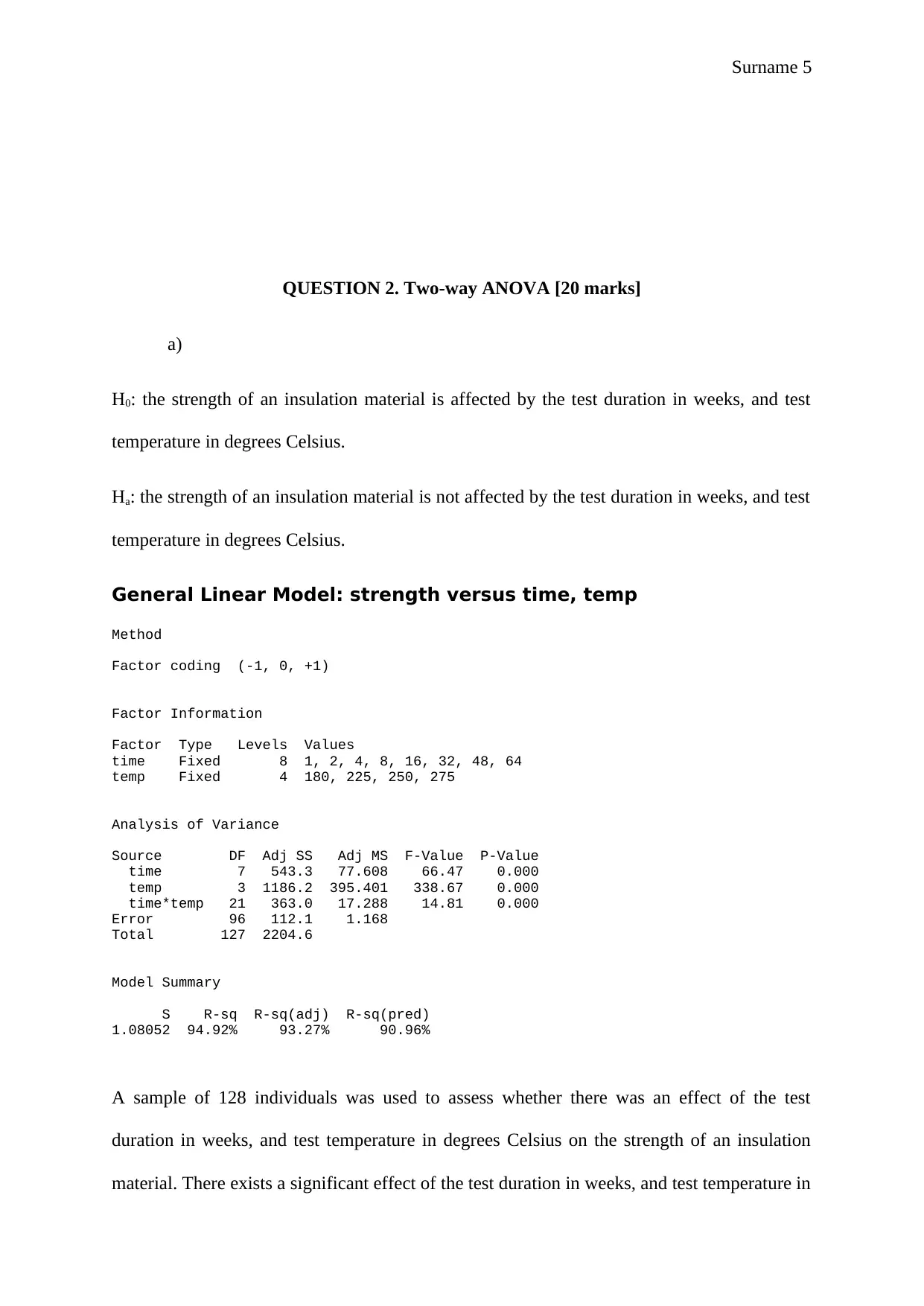
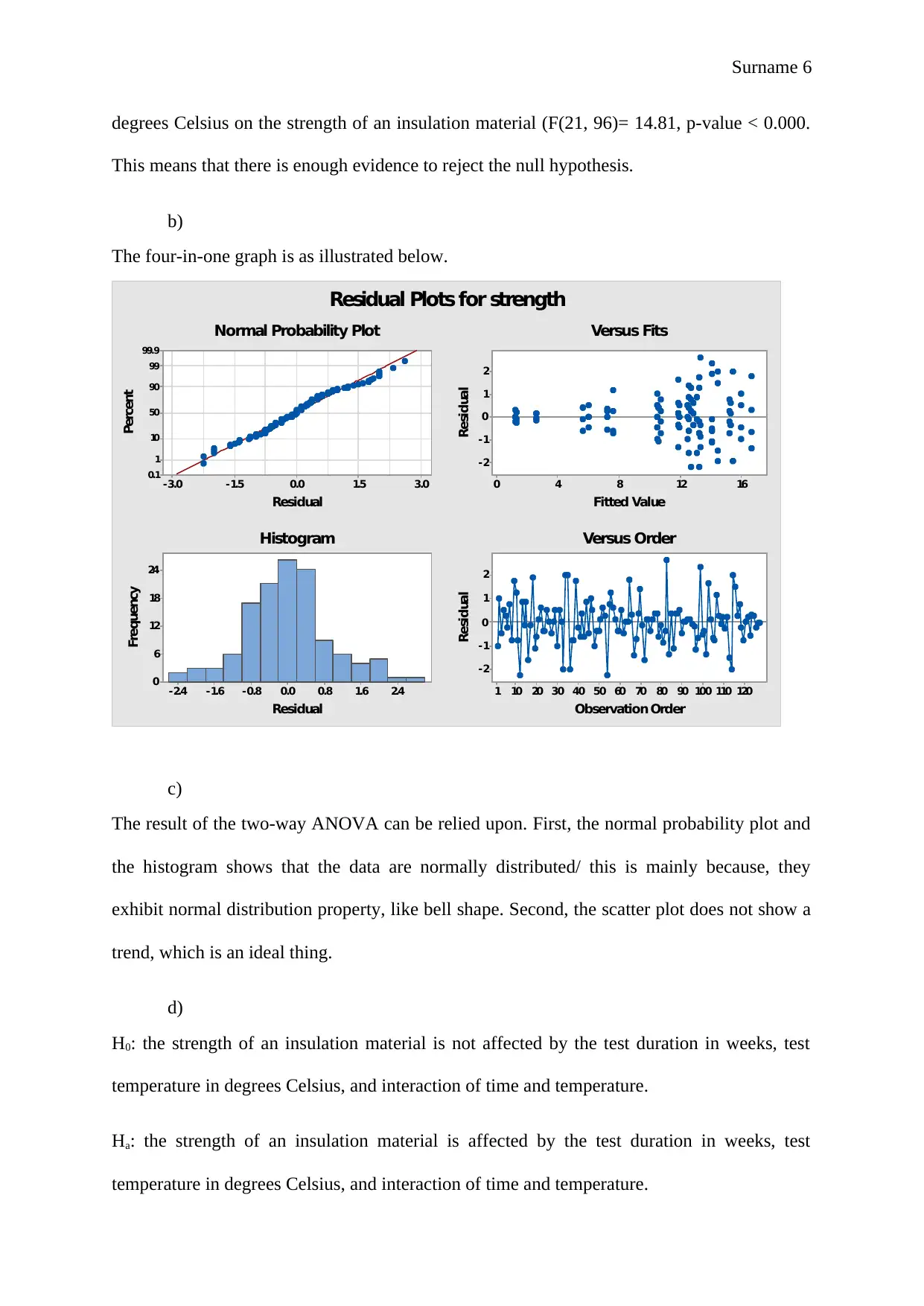
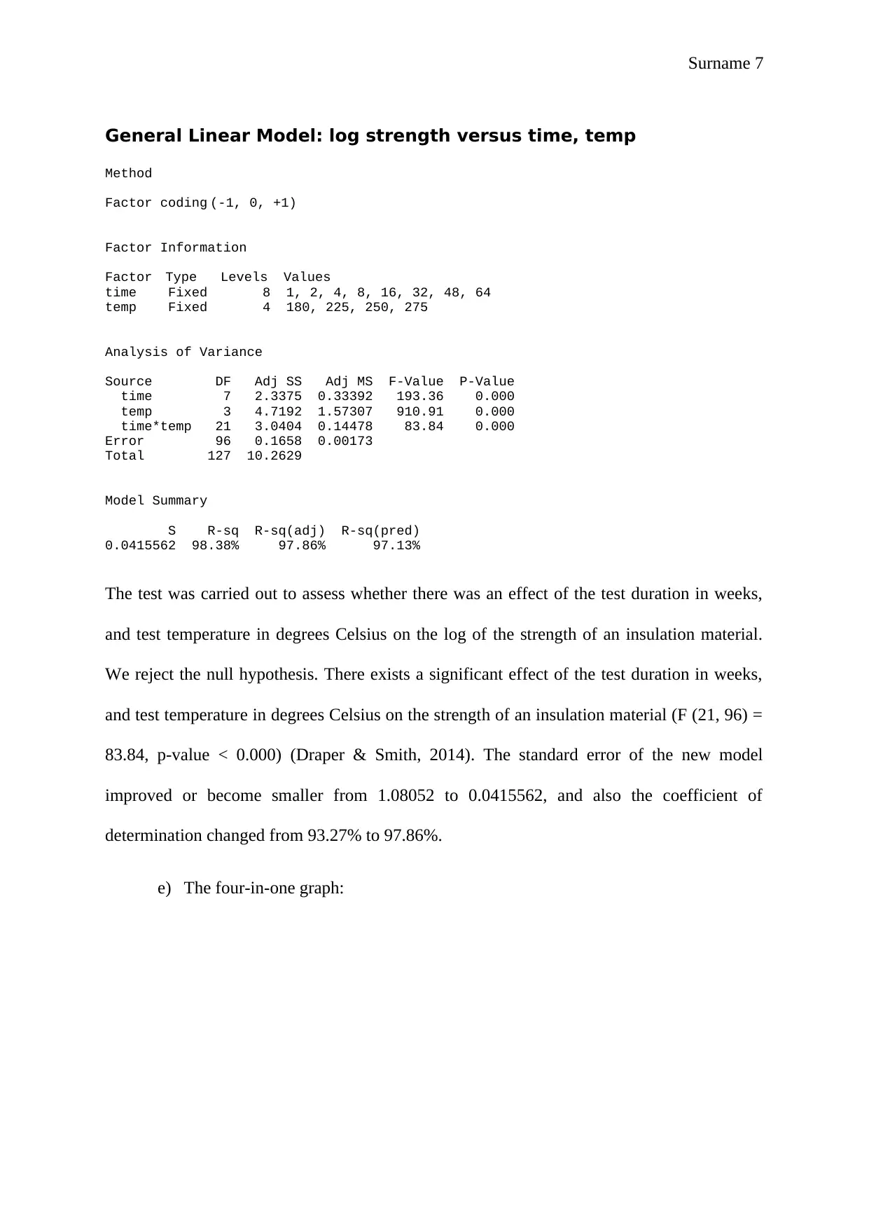
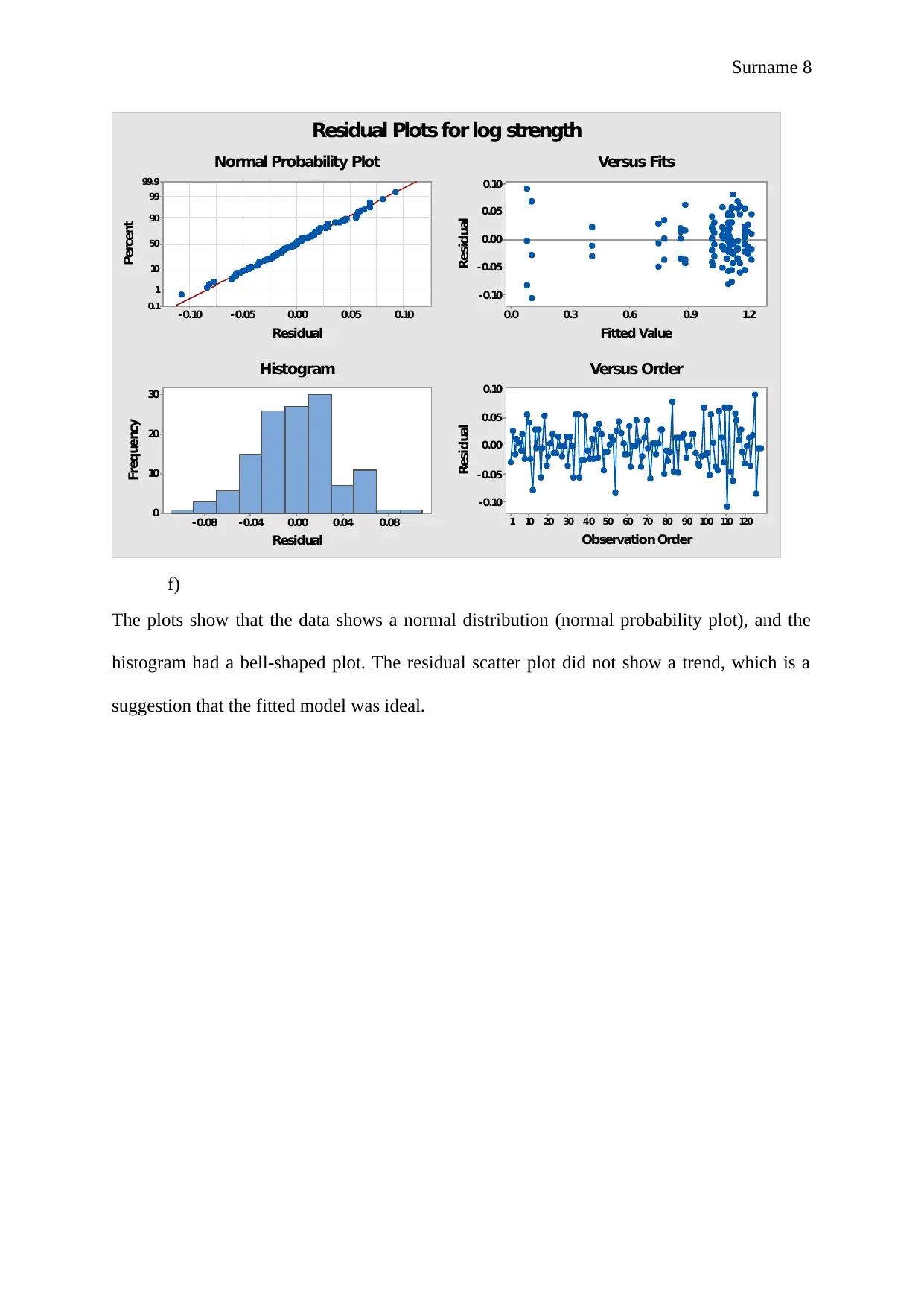
This statistics assignment analyzes data using various statistical methods. The first section applies a two-sample t-test to compare the average weights of football and basketball players, including hypothesis testing and confidence interval calculations. The second section utilizes a two-way ANOVA to assess the effects of test duration and temperature on the strength of an insulation material, examining both the original data and a transformed version. The final section employs multiple linear regression to model lean body mass, considering factors like height, weight, and gender, including model development, variable significance, and interpretation of coefficients. The solution includes model summaries, ANOVA tables, coefficient analysis, and diagnostic plots to validate the models. The assignment also involves the interpretation of the Durbin-Watson statistic, VIF values, and the application of the model to predict lean body mass for specific individuals. References are also provided.

Surname 1
Statistics
Name
The Name of the Class (Course)
Professor (Tutor)
The Name of the School (University)
The City and State where it is located
Date

Surname 2
QUESTION 1. T-test [20 marks]
a)
The most appropriate test is two sample tests, since we are testing the difference between two
independent averages. In this case, the paired t-test cannot be applied since the weight of the
players is not taken from the same sample at two different occasions or time. The sample is
also less than 30, and the population standard deviation is unknown.
Therefore, two sample t-test is the most appropriate test to be applied. The only reason that
can make the test inappropriate is when the data are very skewed. Also, when the sample is
sufficiently large (n > 30), the z-statistics will be used. Lastly, when the sample does not
come from a normally distributed population.
b)
H0: the average weight of a footballer and basketball player is equal, Versus Ha: the average
weight of football players is at least 45 pounds more than the average weight of basketball
players.
Two-Sample T-Test and CI: weight, sport
Two-sample T for weight
Sport N Mean StDev SE Mean
Basketball 19 205.8 12.9 3.0
Football 19 258.8 12.4 2.8
Difference = μ (basketball) - μ (football)
Estimate for difference: -53.00
95% upper bound for difference: -46.07
T-Test of difference = 45 (vs <): T-Value = -23.90 P-Value = 0.000 DF = 35
The results show that there is enough evidence to reject the null hypothesis (t (35) = -23.90, p
< .000) (Moore, et al., 2013). This means that the claim that the average weight of football

Surname 3
players is at least 45 pounds more than the average weight of basketball players is true at the
95% level of confidence.
c)
The 95% upper bound for difference is -46.07, so the C.I is (-46.07, -59.93). This shows that
we are 95% confident that the average population difference of the basket players and the
football players is between the upper and lower bound of the interval.
d)
H0: Football data are normally distributed.
Ha: the football data are not normally distributed.
290280270260250240230
99
95
90
80
70
60
50
40
30
20
10
5
1
Mean 258.8
StDev 12.38
N 19
RJ 0.982
P-Value >0.100
football
Percent
Probability Plot of football
Normal
The results show that RJ = 0.982, p-value > 0.100, which suggests that the null hypothesis
should not be rejected (Yu, et al., 2016). In particular, there is enough evidence to shows that
we cannot conclude that the football data do not follow a normally distribution.
e)
The data are as follows.
footbal transforme

Surname 4
l
d football
weight
245 -1.11417
262 0.259407
255 -0.30619
251 -0.62938
244 -1.19497
276 1.390592
240 -1.51817
265 0.501804
257 -0.14459
252 -0.54858
282 1.875385
256 -0.22539
250 -0.71018
264 0.421005
270 0.905798
275 1.309793
245 -1.11417
275 1.309793
253 -0.46778
The plot is as follows.
210-1-2
5
4
3
2
1
0
Mean 4.616190E-16
StDev 1
N 19
transformed football weight
Frequency
Histogram of transformed football weight
Normal
The plot supports that the data follows a student’s t-distribution since the average is
approximately zero, and the standard deviation is equal to one.

Surname 5
QUESTION 2. Two-way ANOVA [20 marks]
a)
H0: the strength of an insulation material is affected by the test duration in weeks, and test
temperature in degrees Celsius.
Ha: the strength of an insulation material is not affected by the test duration in weeks, and test
temperature in degrees Celsius.
General Linear Model: strength versus time, temp
Method
Factor coding (-1, 0, +1)
Factor Information
Factor Type Levels Values
time Fixed 8 1, 2, 4, 8, 16, 32, 48, 64
temp Fixed 4 180, 225, 250, 275
Analysis of Variance
Source DF Adj SS Adj MS F-Value P-Value
time 7 543.3 77.608 66.47 0.000
temp 3 1186.2 395.401 338.67 0.000
time*temp 21 363.0 17.288 14.81 0.000
Error 96 112.1 1.168
Total 127 2204.6
Model Summary
S R-sq R-sq(adj) R-sq(pred)
1.08052 94.92% 93.27% 90.96%
A sample of 128 individuals was used to assess whether there was an effect of the test
duration in weeks, and test temperature in degrees Celsius on the strength of an insulation
material. There exists a significant effect of the test duration in weeks, and test temperature in

Surname 6
degrees Celsius on the strength of an insulation material (F(21, 96)= 14.81, p-value < 0.000.
This means that there is enough evidence to reject the null hypothesis.
b)
The four-in-one graph is as illustrated below.
3.01.50.0-1.5-3.0
99.9
99
90
50
10
1
0.1
Residual
Percent
1612840
2
1
0
-1
-2
Fitted Value
Residual
2.41.60.80.0-0.8-1.6-2.4
24
18
12
6
0
Residual
Frequency
1201101009080706050403020101
2
1
0
-1
-2
Observation Order
Residual
Normal Probability Plot Versus Fits
Histogram Versus Order
Residual Plots for strength
c)
The result of the two-way ANOVA can be relied upon. First, the normal probability plot and
the histogram shows that the data are normally distributed/ this is mainly because, they
exhibit normal distribution property, like bell shape. Second, the scatter plot does not show a
trend, which is an ideal thing.
d)
H0: the strength of an insulation material is not affected by the test duration in weeks, test
temperature in degrees Celsius, and interaction of time and temperature.
Ha: the strength of an insulation material is affected by the test duration in weeks, test
temperature in degrees Celsius, and interaction of time and temperature.

Surname 7
General Linear Model: log strength versus time, temp
Method
Factor coding (-1, 0, +1)
Factor Information
Factor Type Levels Values
time Fixed 8 1, 2, 4, 8, 16, 32, 48, 64
temp Fixed 4 180, 225, 250, 275
Analysis of Variance
Source DF Adj SS Adj MS F-Value P-Value
time 7 2.3375 0.33392 193.36 0.000
temp 3 4.7192 1.57307 910.91 0.000
time*temp 21 3.0404 0.14478 83.84 0.000
Error 96 0.1658 0.00173
Total 127 10.2629
Model Summary
S R-sq R-sq(adj) R-sq(pred)
0.0415562 98.38% 97.86% 97.13%
The test was carried out to assess whether there was an effect of the test duration in weeks,
and test temperature in degrees Celsius on the log of the strength of an insulation material.
We reject the null hypothesis. There exists a significant effect of the test duration in weeks,
and test temperature in degrees Celsius on the strength of an insulation material (F (21, 96) =
83.84, p-value < 0.000) (Draper & Smith, 2014). The standard error of the new model
improved or become smaller from 1.08052 to 0.0415562, and also the coefficient of
determination changed from 93.27% to 97.86%.
e) The four-in-one graph:

Surname 8
0.100.050.00-0.05-0.10
99.9
99
90
50
10
1
0.1
Residual
Percent
1.20.90.60.30.0
0.10
0.05
0.00
-0.05
-0.10
Fitted Value
Residual
0.080.040.00-0.04-0.08
30
20
10
0
Residual
Frequency
1201101009080706050403020101
0.10
0.05
0.00
-0.05
-0.10
Observation Order
Residual
Normal Probability Plot Versus Fits
Histogram Versus Order
Residual Plots for log strength
f)
The plots show that the data shows a normal distribution (normal probability plot), and the
histogram had a bell-shaped plot. The residual scatter plot did not show a trend, which is a
suggestion that the fitted model was ideal.

Surname 9
Question 3. Multiple Linear Regression [20 marks]
a)
The matrix scatters plot is as illustrated below.
The plot shows that the male might have a higher lean body mass than that of female athletics
(Mayorga & Gleicher, 2013). This is indicated by the scatter plot being distinctively higher in
both cases. Also, the interaction of gender might be vital in the development of the model. the
height shows a positive association with the independent variable, which means that its
inclusion in the model is important. Similar, relationship exists between the height and lean
body mass since the scatter plot spread from bottom left to top right. Thus, the inclusion of
these variables will be vital to assess whether they are significantly associated with lbm.
b)
The model summary is as summarized below.
Model Summaryb
Model R R Square
Adjusted R
Square
Std. Error of the
Estimate Durbin-Watson
1 .982a .965 .964 2.46880 1.535
a. Predictors: (Constant), interaction of weight and gender, height, weight, Gender,
interaction of height and gender
b. Dependent Variable: lean body mass

Surname 10
ANOVAa
Model Sum of Squares df Mean Square F Sig.
1 Regression 33142.224 5 6628.445 1087.524 .000b
Residual 1194.618 196 6.095
Total 34336.841 201
a. Dependent Variable: lean body mass
b. Predictors: (Constant), interaction of weight and gender, height, weight, Gender, interaction of
height and gender
Coefficientsa
Model
Unstandardized Coefficients
Standardized
Coefficients
t Sig.B Std. Error Beta
1 (Constant) 2.551 6.112 .417 .677
height .094 .043 .070 2.202 .029
weight .534 .032 .569 16.562 .000
Gender -14.029 8.913 -.538 -1.574 .117
interaction of height and
gender .054 .060 .388 .912 .363
interaction of weight and
gender .177 .042 .571 4.228 .000
a. Dependent Variable: lean body mass
The developed model is significant (F (5, 196) = 1087.524, p-value < .000). The model is:
lbm =2.551+ 0.094(ht) + 0.534(wt) -14.029(gender) + 0.054 (ht*gender) + 0.177(wt*gender)
However, not all the predictor’s variables are significant. Therefore, those with a p-value >
0.05, were deleted and a second linear regression model developed (Chatterjee & Hadi.,
2015).
c)

Surname 11

Surname 12
The histogram indicates that the residual distribution is not approximately normal since the
standard deviation is 0.987. Also, the PP plot of the standardized residual indicate that there
d)
A new model was run, using only significant dependent variables.
Model Summaryb
Model R R Square
Adjusted R
Square
Std. Error of the
Estimate Durbin-Watson
1 .982a .964 .963 2.50638 1.530
a. Predictors: (Constant), interaction of weight and gender, height, weight
b. Dependent Variable: lean body mass
ANOVAa
Model Sum of Squares df Mean Square F Sig.
1 Regression 33093.022 3 11031.007 1755.994 .000b
Residual 1243.820 198 6.282
Total 34336.841 201
a. Dependent Variable: lean body mass
b. Predictors: (Constant), interaction of weight and gender, height, weight
Coefficientsa