Elementary Statistics: Data Analysis, Probability, and Interpretation

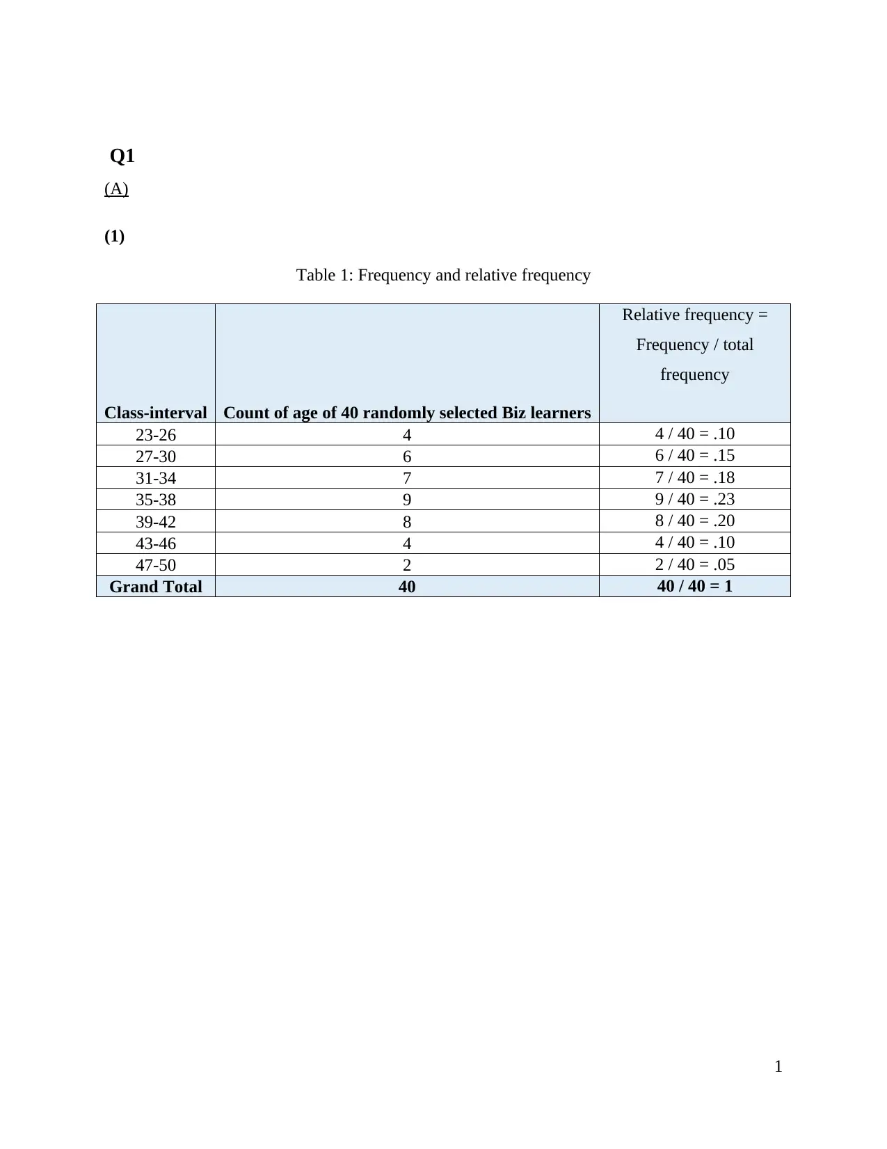
This document provides a detailed solution to an elementary statistics assignment. The assignment covers various statistical concepts, including frequency distribution, mean, mode, median, and standard deviation calculations. It explores data analysis through tables and charts, such as frequency charts and cumulative frequency charts. The solution also includes calculations of the coefficient of variation and analysis of probability through interpreting loyalty test results. The document is well-structured, providing step-by-step calculations and interpretations, making it a valuable resource for students studying statistics. It provides a good understanding of descriptive statistics, probability and data interpretation.

ELEMENTARY STATISTICS

TABLE OF CONTENTS
Q1.....................................................................................................................................................1
(A)...............................................................................................................................................1
(1).......................................................................................................................................1
(2).......................................................................................................................................2
(3).......................................................................................................................................2
(4).......................................................................................................................................3
(b)................................................................................................................................................4
(1).......................................................................................................................................4
Q 2....................................................................................................................................................6
(A)...............................................................................................................................................6
(1).......................................................................................................................................6
Q3...................................................................................................................................................10
(A)....................................................................................................................................10
(B)....................................................................................................................................10
©......................................................................................................................................10
(D)....................................................................................................................................11
(E)....................................................................................................................................11
(F)....................................................................................................................................11
REFERENCES..............................................................................................................................12
Table 1Frequency and relative frequency........................................................................................1
Table 2Cumulative frequency table.................................................................................................2
Table 3Input to prepare Ogive chart................................................................................................3
Table 4Input table............................................................................................................................4
Table 5Mean calculation..................................................................................................................4
Table 6Standard deviation calculation.............................................................................................5
Table 7Average of weight...............................................................................................................6
Table 8Median of weight of bags....................................................................................................7

Table 9Mode of weight of bags.......................................................................................................8
Table 10Standard deviation of weight of bags................................................................................8
Figure 1Frequency chart..................................................................................................................2
Figure 2Cumulative frequency chart...............................................................................................3
Figure 3Loayalty test results..........................................................................................................10

Q1
(A)
(1)
Table 1: Frequency and relative frequency
Class-interval Count of age of 40 randomly selected Biz learners
Relative frequency =
Frequency / total
frequency
23-26 4 4 / 40 = .10
27-30 6 6 / 40 = .15
31-34 7 7 / 40 = .18
35-38 9 9 / 40 = .23
39-42 8 8 / 40 = .20
43-46 4 4 / 40 = .10
47-50 2 2 / 40 = .05
Grand Total 40 40 / 40 = 1
1

(2)
Figure 1Frequency chart
Frequency chart is the one of the most important tool because it reflect the clasification of
data into multiple categories. By using this tool it can be identified that in which group there are
large number of observations or trend that is seen most of times in the observation. Group 35 to
38 have highest proportiion with 9 observations out of total numebr of observations.
(3)
Table 2Cumulative frequency table
Class-interval
Count of age
of 40
randomly
selected Biz
learners
Cumulative
frequency
23-26 4 4
27-30 6 10
31-34 7 17
2

35-38 9 26
39-42 8 34
43-46 4 38
47-50 2 40
Total 40
Figure 2Cumulative frequency chart
(4)
Particulars
Age of Biz
learners
Quartile 1 31
Quartile 2 (Median) 36
Quartile 3 39
On evaluation of Ogive chart given above it is identified that value of Q1 is 31, Q2 is 36
and Q3 is 39 respectively.
3

(b)
(1)
Table 3Input table
1
Wet Market
A
Wet Market
B
2 23 20
3 21 20
4 24 21
5 23 22
6 24 22
7 23 23
8 22 21
9 22 21
10 23 23
Table 4Mean calculation
Particulars Wet Market A Wet Market B
Total prices of Seabass
(RM/kg)
205 193
Number of observations 10 10
Mean (RM/kg) 20.5 19.3
Average is the one of the most important tool that reflect overall performance of the
variable (Amrhein, Trafimow and Greenland., 2019). Mean value of Wet market A is 20.5 and
same of market B is 19.3 and, on this basis, it can be said that in both wet market sale of almost
same quantity is made across sample units.
4

Table 5: Standard deviation calculation
1 Wet
Market A X – Mean (X – Mean)^2
2 23 2.5 6.25
3 21 0.5 0.25
4 24 3.5 12.25
5 23 2.5 6.25
6 24 3.5 12.25
7 23 2.5 6.25
8 22 1.5 2.25
9 22 1.5 2.25
10 23 2.5 6.25
205 20.5 54.25
Variance = 54.25 / 10
= 5.425
Standard deviation = SQRT(Variance)
=√5.425
= 2.33
1 Wet
Market b X – Mean (X – Mean)^2
2 20 0.7 0.49
3 20 0.7 0.49
4 21 1.7 2.89
5 22 2.7 7.29
6 22 2.7 7.29
7 23 3.7 13.69
8 21 1.7 2.89
9 21 1.7 2.89
10 23 3.7 13.69
Total 193 19.3 51.61
Variance = 51.61 / 10
= 5.161
Standard deviation = SQRT(Variance)
=√5.161
5

= 2.27
Standard deviation is the tool that indicate the extent to which deviation happened in the
value of the variable relative to mean value (Mishra and et.al., 2019). Standard deviation of wet
market A is 2.33 and same of market B is 2.27 and, on this basis, it can be said that value is not
much deviating from mean value in both market. Mean value are almost nearby to each other and
on this basis, it can be said that across both markets same trends prevailed.
B (ii) coefficient of variation
Coefficient of variation = (Std dev / Mean) x 100
Wet market A: (2.33 / 20.5) * 100 = 11.36
Wet market B: (2.27 / 19.3) * 100 = 11.76
Q 2
(A)
(1) Mean
Table 6: Average of weight
Weight of
bags
1 5.01
2 4.98
3 5.02
4 5
5 4.99
6 5
7 4.97
8 5.02
9 5
10 5.01
11 5.01
12 5
6

Total 60.01
Number
N 12
Average 5.00
Mean = Sum of observations/ Number of observations
= 60.01/12 = 5 kg
Mean value of the variable is 5 which means that on an average basis weight of the rice
5KG in most of bags.
2. Mode
Table 8: Mode of weight of bags
Weight of bags Count of Weight of bags / frequency
4.97 1
4.98 1
4.99 1
5 4
5.01 3
5.02 2
Grand Total 12
Mode value is 5 because it repeated 4 times in the dataset which is high in the number.
3. Median
Table 9: Median of weight of bags
Weight
of bags
1 4.97
2 4.98
3 4.99
4 5
5 5
6 5
7 5
8 5.01
9 5.01
7

10 5.01
11 5.02
12 5.02
Median Position = (n+1)/2 when number of observation is odd
= (12+1)/2 = 6.5
Value of 6 + value of 7th item / 2
= (5+ 5) / 2 = 5 kg
In the above table it can be seen that median value is 5 which means that it is the value that
divide entire dataset into two parts.
4. Variance
Weight
of bags
(X
X – Mean (X –
Mean)^2
1 5.01 0.01 0.0001
2 4.98 -0.02 0.0004
3 5.02 0.02 0.0004
4 5 0.00 0
5 4.99 -0.01 0.0001
6 5 0.00 0
7 4.97 -0.03 0.0009
8 5.02 0.02 0.0004
9 5 0.00 0
10 5.01 0.01 0.0001
11 5.01 0.01 0.0001
12 5 0.00 0
Total 60.01 0.0025
Variance = SUM (X- Mean) ^2/ Number of observations
8

= 0.0025/12
= 0.0002
5. Standard deviation
Standard deviation = SQRT (Variance)
= √0. 0002
=0.0144
Standard deviation value is 0.0144 which is quite low and indicate that variables values are
very close to the mean value in the dataset.
(b) Stating the type of distribution using location relationship
By doing assessment, it has identified that information pertaining to weight of bags fall
under the category of individual data series. For analysing such data prominently descriptive
statistics tool has been applied. Moreover, descriptive statistics clearly exhibit average, median,
variances etc pertaining to given data set.
9