University Statistics Assignment: STM4PSD, Week 11

This statistics assignment solution addresses several statistical problems. The first problem involves comparing two weight loss programs (X and Y) using a paired t-test with R commands and outputs, including hypothesis testing, confidence intervals, and p-value analysis. The second problem focuses on comparing the performance of two machines manufacturing memory chips using the prop.test function in R, examining proportions, confidence intervals, and p-values. The third problem analyzes the relationship between the age and circumference of orange trees using scatterplots, boxplots, and linear regression models in R, covering model fitting, coefficient interpretation, and prediction intervals. The assignment includes detailed R code, outputs, and interpretations for each problem, providing a comprehensive guide for statistical analysis.

Running Head: STATISTICS ASSIGNMENT
Statistics Assignment
Name of the Student
Name of the University
Student ID

1STATISTICS ASSIGNMENT
Table of Contents
Answer 1....................................................................................................................................3
Part A.....................................................................................................................................3
Part B......................................................................................................................................3
Part C......................................................................................................................................3
Part D.....................................................................................................................................3
Part E......................................................................................................................................4
Answer 2....................................................................................................................................4
Part A.....................................................................................................................................5
Part i...................................................................................................................................5
Part ii..................................................................................................................................5
Part iii.................................................................................................................................5
Part B......................................................................................................................................5
Part C......................................................................................................................................5
Part D.....................................................................................................................................6
Answer 3....................................................................................................................................6
Part A.....................................................................................................................................6
Part B......................................................................................................................................6
Part C......................................................................................................................................7
Part D.....................................................................................................................................8
Part E......................................................................................................................................9

2STATISTICS ASSIGNMENT
Part F......................................................................................................................................9
Part G.....................................................................................................................................9
Part H.....................................................................................................................................9
Part I.......................................................................................................................................9
Part J.......................................................................................................................................9
Part K...................................................................................................................................10
Part I.....................................................................................................................................10

3STATISTICS ASSIGNMENT
Answer 1
Part A
Null Hypothesis (H0): X ≤ Y
Alternate Hypothesis (HA): X > Y
Part B
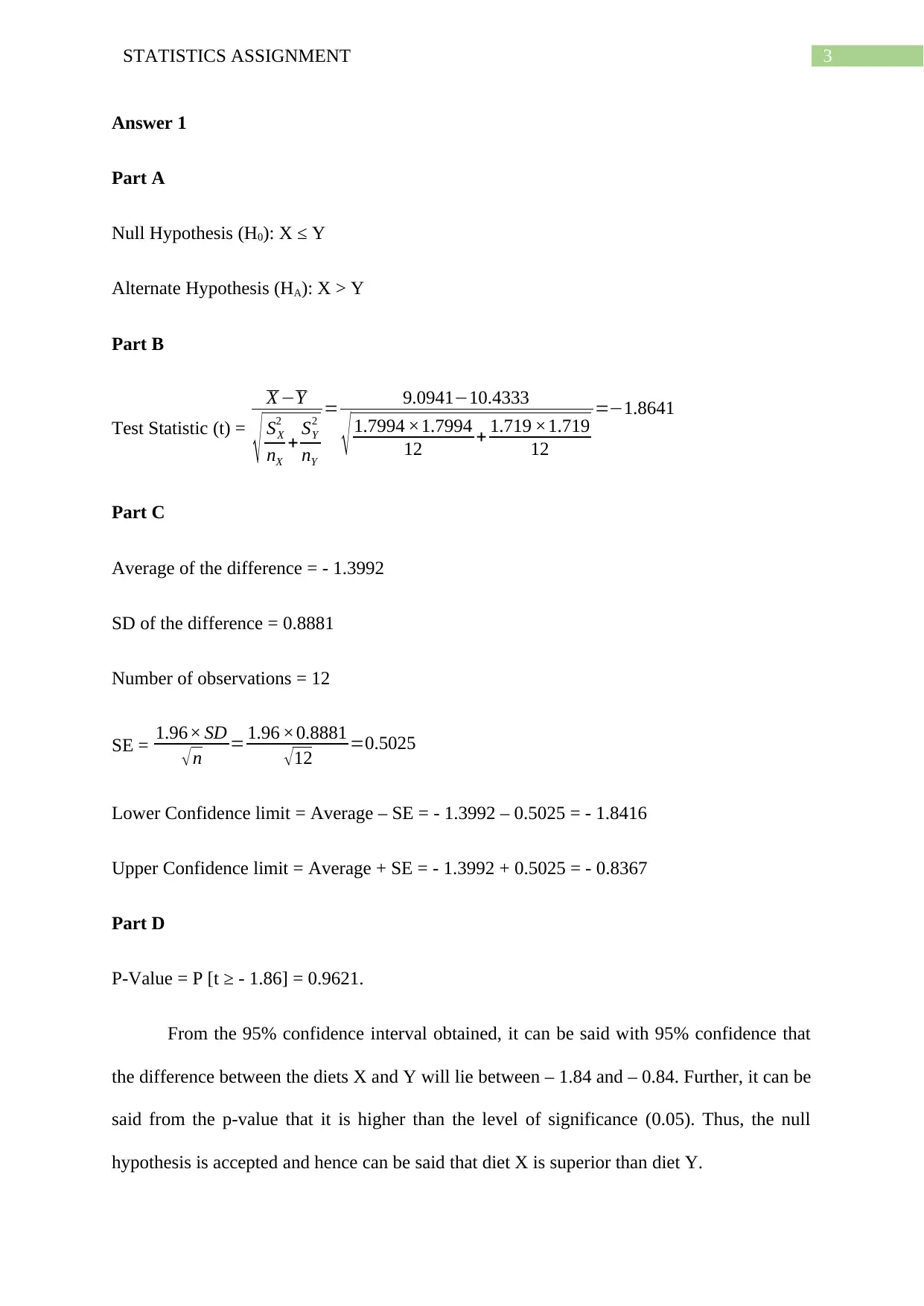
Test Statistic (t) =
X −Y
√ SX
2
nX
+ SY
2
nY
= 9.0941−10.4333
√ 1.7994 ×1.7994
12 + 1.719 ×1.719
12
=−1.8641
Part C
Average of the difference = - 1.3992
SD of the difference = 0.8881
Number of observations = 12
SE = 1.96× SD
√n = 1.96 ×0.8881
√12 =0.5025
Lower Confidence limit = Average – SE = - 1.3992 – 0.5025 = - 1.8416
Upper Confidence limit = Average + SE = - 1.3992 + 0.5025 = - 0.8367
Part D
P-Value = P [t ≥ - 1.86] = 0.9621.
From the 95% confidence interval obtained, it can be said with 95% confidence that
the difference between the diets X and Y will lie between – 1.84 and – 0.84. Further, it can be
said from the p-value that it is higher than the level of significance (0.05). Thus, the null
hypothesis is accepted and hence can be said that diet X is superior than diet Y.

4STATISTICS ASSIGNMENT
Part E
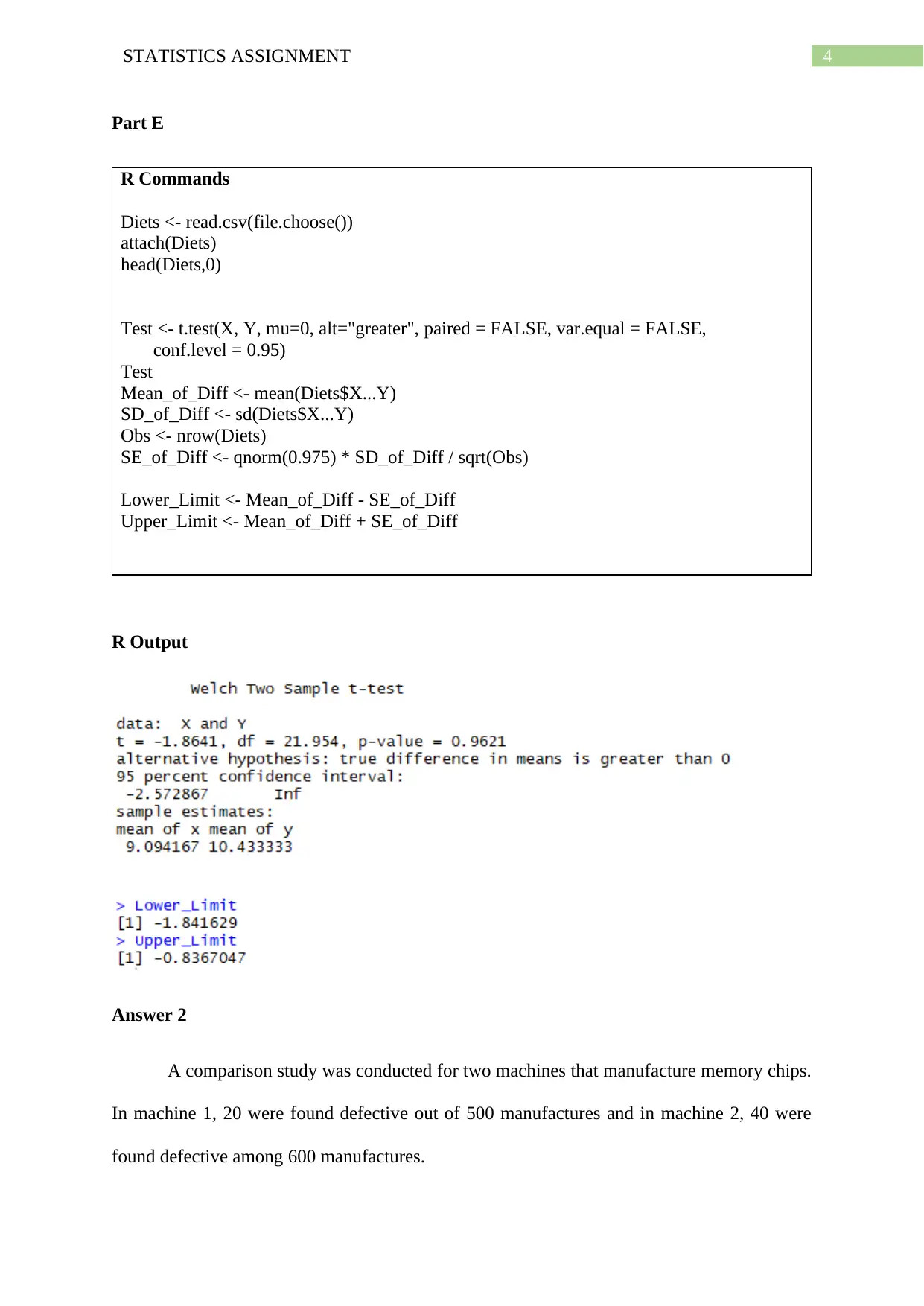
R Commands
Diets <- read.csv(file.choose())
attach(Diets)
head(Diets,0)
Test <- t.test(X, Y, mu=0, alt="greater", paired = FALSE, var.equal = FALSE,
conf.level = 0.95)
Test
Mean_of_Diff <- mean(Diets$X...Y)
SD_of_Diff <- sd(Diets$X...Y)
Obs <- nrow(Diets)
SE_of_Diff <- qnorm(0.975) * SD_of_Diff / sqrt(Obs)
Lower_Limit <- Mean_of_Diff - SE_of_Diff
Upper_Limit <- Mean_of_Diff + SE_of_Diff
R Output
Answer 2
A comparison study was conducted for two machines that manufacture memory chips.
In machine 1, 20 were found defective out of 500 manufactures and in machine 2, 40 were
found defective among 600 manufactures.

5STATISTICS ASSIGNMENT
To test the difference in proportions, the R function prop.test has been used. The code
and the results are given as follows:
Result <- prop.test (x = c(480, 560), n = c(500, 600))
Result
Part A
Part i
The estimate to p1 is 0.96 and the estimate to p2 is 0.93.
Part ii
The approximate 95% confidence interval for p1− p2 is (-0.0015, 0.0548)
Part iii
The p-value for the test comparing p1 and p2 is 0.07093
Part B
The p-value is greater than the level of significance (α = 0.05). Thus, it can be said that the
proportions are equal. There is not enough evidence to reject the hypothesis that the
proportions are equal.
Part C
The confidence interval ranges from a negative to a positive range and both the upper
and the lower values are quite close to zero. Thus, it cannot be said that one machine
performs better than the other.

6STATISTICS ASSIGNMENT
Part D
From all the findings reported above, it can be said that there is no significant
difference between the performance of the two machines.
Answer 3
Part A
R Code
##-----------------Scatterplot--------------------##
Scatterplot <- scatter.smooth(age, circumference, span = 2/3, degree = 1,
family = c("symmetric", "gaussian"), pch = 19,
main = "Scatterplot of Age and Circumference of Trees")
Part B
R Codes
##-----------------Boxplot--------------------##

7STATISTICS ASSIGNMENT
par(mfrow = c(1,2))
boxplot(age, main = "Boxplot of Age",
xlab = "Age", ylab = "Days")
boxplot(circumference, main = "Boxplot of Circumference",
xlab = "Circumference", ylab = "Unit (in mm)")
It can be seen clearly from the boxplots, that there are no outliers to the data.
Part C
R Codes
##-----------------Least Square Regression--------------------##
lm.model <- lm(circumference ~ age, data = Orange)
summary(lm.model)
R Output

8STATISTICS ASSIGNMENT
Part D
R Codes
par(mfrow = c(1,2))
plot(lm.model, pch = 19, lwd = 2)

9STATISTICS ASSIGNMENT
The residuals vs fitted plot is completely random and also the normal Q-Q plot is
almost linear. This indicates that the data follows the assumption of normality. Thus, there
are no violations of the linear regression model.
Part E
From the R output, it can be seen that the r squared value for the regression is 0.8345.
This indicates that 83.45% of the variability in the dependent variable can be explained by the
independent variable. Thus, the model is a good fit.
Part F
The estimate for the coefficient of age is 0.1068 and that of the intercept is 17.3997.
Part G
It can be seen from the R output that the p-value for the age coefficient is less than the
level of significance (0.05). Thus, the null hypothesis is accepted.
Part H
It can be seen from the R output that the p-value for the intercept coefficient is more
than the level of significance (0.05). Thus, the null hypothesis is rejected.
Part I
R Codes and Output
Part J

10STATISTICS ASSIGNMENT
Circumference = 17.3997 + (0.1068 * Age) = 17.3997 + (0.1068 * 540) = 75.07 mm
Part K
R Codes and Output
A prediction interval gives an insight about the distribution of the values whereas, a
confidence interval gives us an insight about the location that is likely for the two population
parameter. That is why, the two intervals are different.
Part I
There has been a positive relationship between the circumference of the orange trees
and their age. Further, the regression has been found a good fit and significant as well. Thus,
there is enough evidence to conclude that with the increase in age, the circumference of the
orange trees increases.