Statistics for Management: Analysis of Economic and Business Data

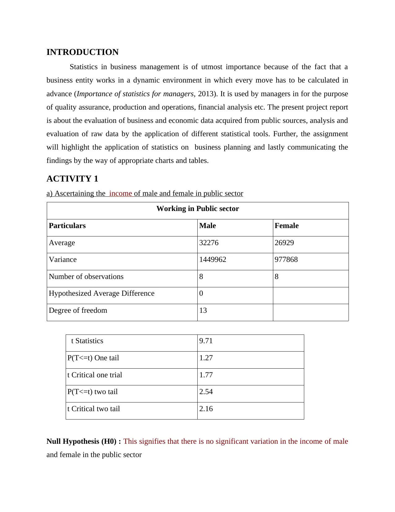
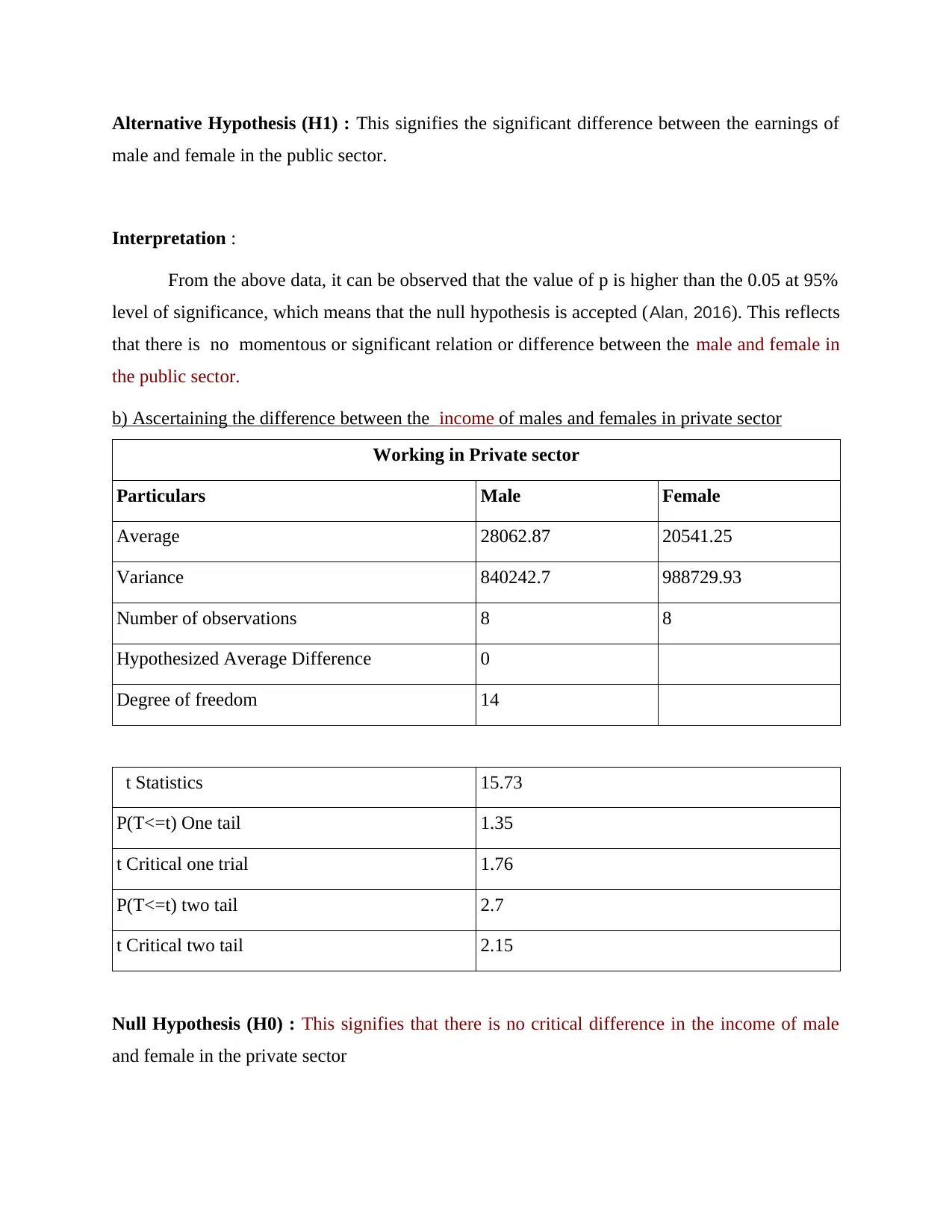
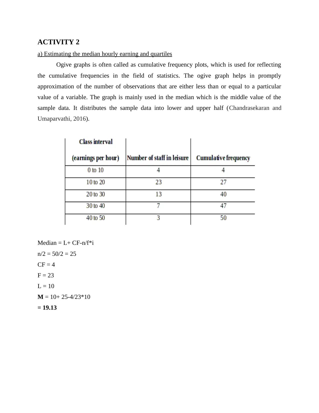
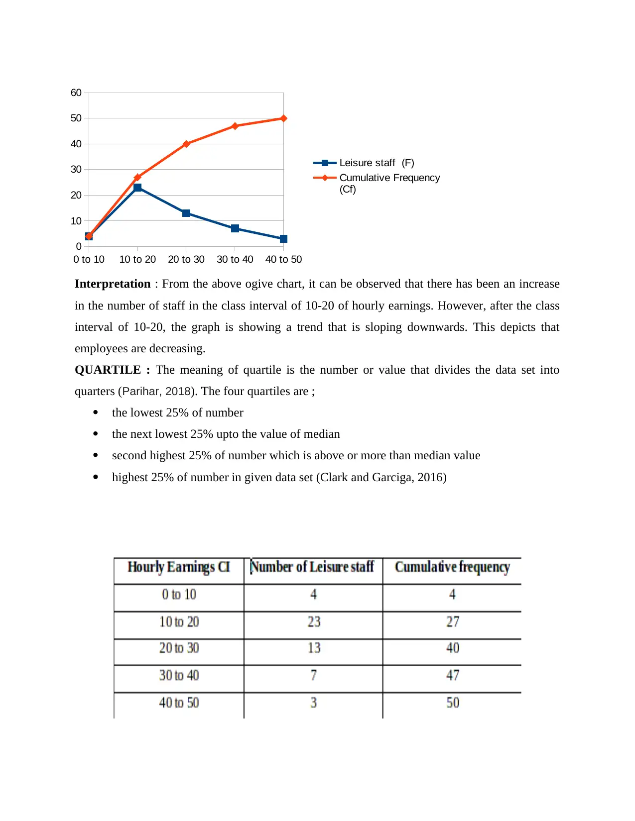
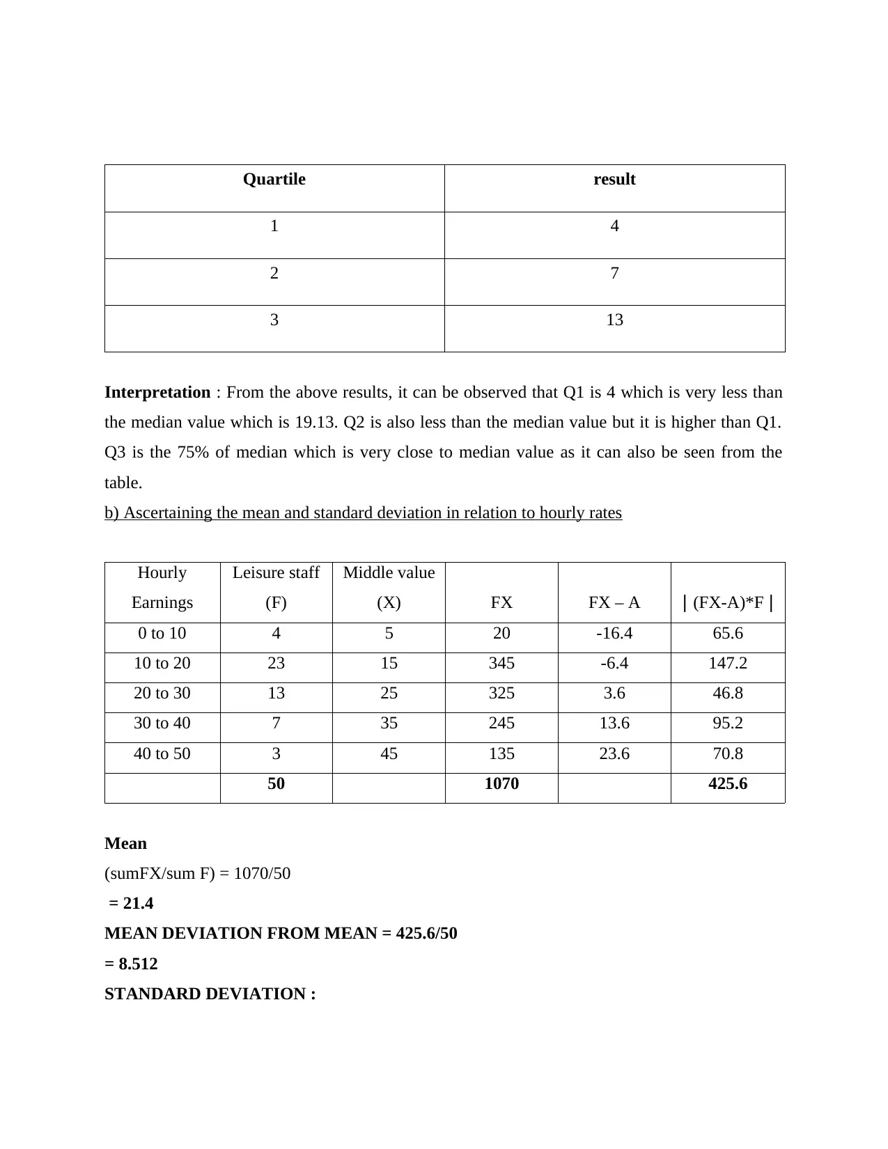
This report presents a statistical analysis of economic and business data, utilizing various statistical tools and techniques. The report begins with an introduction to the importance of statistics in business management, followed by an analysis of income differences between males and females in both public and private sectors, along with the presentation of income trends from 2009 to 2016. The report also includes the determination of annual growth rates for different groups. Activity 2 focuses on estimating median hourly earnings, quartiles, mean, and standard deviation, with a comparison of statistics between two different regions. Activity 3 involves calculating the Economic Order Quantity (EOQ), inventory policy costs, and service levels. Finally, Activity 4 presents charts for RPI, CPI, and CHIP from 2007 to 2017, along with an Ogive chart. The report concludes with a summary of the findings and relevant references.

Statistics For Management

Table of Contents
..........................................................................................................................................................3
INTRODUCTION...........................................................................................................................4
ACTIVITY 1 ...................................................................................................................................4
a) Ascertaining the earnings of male and female in public sector..............................................4
b) Ascertaining the difference between the earnings of males and females in private sector.....5
c) Presentation of the earnings of men and women from the period of 2009 to 2016...............5
d) Determining the annual growth rate of all four groups..........................................................8
ACTIVITY 2....................................................................................................................................9
a) Estimating the median hourly earning and quartiles...............................................................9
b) Ascertaining the mean and standard deviation in relation to hourly rates............................11
Comparison of the statistics of two different regions...............................................................12
ACTIVITY 3 .................................................................................................................................13
a) Calculating economic order quantity (EOQ)........................................................................13
b) Occurrence of cost and cost..................................................................................................14
c) Calculating inventory policy cost........................................................................................14
d) Identifying current service level ..........................................................................................14
e) Ascertaining the re-order level..............................................................................................14
ACTIVITY 4 .................................................................................................................................15
a) Formation of charts for RPI, CPI and CHIP from 2007- 2017.............................................15
b) Presentation of the Ogive chart for the cumulative % of leisure staff and hourly earnings. 17
CONCLUSION .............................................................................................................................17
REFERENCES..............................................................................................................................18
Books and Journals...................................................................................................................18

INTRODUCTION
Statistics in business management is of utmost importance because of the fact that a
business entity works in a dynamic environment in which every move has to be calculated in
advance (Importance of statistics for managers, 2013). It is used by managers in for the purpose
of quality assurance, production and operations, financial analysis etc. The present project report
is about the evaluation of business and economic data acquired from public sources, analysis and
evaluation of raw data by the application of different statistical tools. Further, the assignment
will highlight the application of statistics on business planning and lastly communicating the
findings by the way of appropriate charts and tables.
ACTIVITY 1
a) Ascertaining the income of male and female in public sector
Working in Public sector
Particulars Male Female
Average 32276 26929
Variance 1449962 977868
Number of observations 8 8
Hypothesized Average Difference 0
Degree of freedom 13
t Statistics 9.71
P(T<=t) One tail 1.27
t Critical one trial 1.77
P(T<=t) two tail 2.54
t Critical two tail 2.16
Null Hypothesis (H0) : This signifies that there is no significant variation in the income of male
and female in the public sector

Alternative Hypothesis (H1) : This signifies the significant difference between the earnings of
male and female in the public sector.
Interpretation :
From the above data, it can be observed that the value of p is higher than the 0.05 at 95%
level of significance, which means that the null hypothesis is accepted (Alan, 2016). This reflects
that there is no momentous or significant relation or difference between the male and female in
the public sector.
b) Ascertaining the difference between the income of males and females in private sector
Working in Private sector
Particulars Male Female
Average 28062.87 20541.25
Variance 840242.7 988729.93
Number of observations 8 8
Hypothesized Average Difference 0
Degree of freedom 14
t Statistics 15.73
P(T<=t) One tail 1.35
t Critical one trial 1.76
P(T<=t) two tail 2.7
t Critical two tail 2.15
Null Hypothesis (H0) : This signifies that there is no critical difference in the income of male
and female in the private sector

Alternative Hypothesis (H1) : This signifies the significant variation between the income of
men and women in the private sector.
Interpretation : It can be seen that the numerical quantity of p is higher than 0.05 and t is 1.35
which means that null hypothesis is accepted (Calculator, 2015). This shows that the income of
male and female both in the privately held sector does not reflects significant difference in their
earnings respectively.
c) Presentation of the income of female and male from the period of 2009 to 2016
Income of men in private and public sector annually
Years Public Private
2009 30638 27632
2010 31264 27000
2011 31380 27233
2012 31816 27705
2013 32541 28201
2014 32878 28442
2015 33685 28881
2016 34011 29679

Interpretation : From the above graph, it can be observed that the both men has experienced
increase in their income from 2009 to 2016 and this increase has been proportionately similar in
both the sectors. The data has showed that income in the private sector for men ranges from
above 25000 to below 30000 whereas in the public sector it ranges from 30000 to 35000. It can
be said that there has been constant increase in both the sectors.

Income of women in private and public sector annually
Years Public Private
2009 25224 19551
2010 26113 19532
2011 26470 19565
2012 26636 20313
2013 27338 20698
2014 27705 21017
2015 27905 21403
2016 28053 22251

Interpretation : The above line chart reflects the income of women in civil service sector and
economic sector over the period of 8 years. From the graph, it can be interpreted that women are
getting lesser pay than the men in both the sectors. Also, it can be said that women in private
sector are earning very less as compared to women in the public sector.
d) Determining the annual growth rate of all four groups

Growth Rate of income of females in public sector : The growth rate in the public sector for
women has declined during the 8 years as it can be seen that in the year 2010, it was 3.5 %
whereas in the year 2016, it was only 0.5% which shows significant decline in the growth rate of
the women's income in the public sector.
Growth Rate of income of females in private sector : The case is different in the private sector
for the women. The income of women in the private sector has seen a rise as it was negative 0.1
% in 2010 which kept on increasing till the year 2012 to 3.8 % which further declined and then
again arose in year 2016 to 4%.
Growth Rate of income of males in public sector : Men has experience rise in their income
continuously ever since 2009 when it was 30368 to 34011 in the year 2016. However, the growth
rate is not stable and is fluctuating.
Rate of growth in male's income in private or economic sector : The rate of growth in the
income of men in private sector has seen growth as it was -1.3% in the year 2010 as compared to
2.8% in the year 2016. However, the growth rate has not stable in this sector.

ACTIVITY 2
a) Estimating the median hourly earning and quartiles
Ogive graphs is often called as cumulative frequency plots, which is used for reflecting
the cumulative frequencies in the field of statistics. The ogive graph helps in promptly
approximation of the number of observations that are either less than or equal to a particular
value of a variable. The graph is mainly used in the median which is the middle value of the
sample data. It distributes the sample data into lower and upper half (Chandrasekaran and
Umaparvathi, 2016).
Median = L+ CF-n/f*i
n/2 = 50/2 = 25
CF = 4
F = 23
L = 10
M = 10+ 25-4/23*10
= 19.13

Interpretation : From the above ogive chart, it can be observed that there has been an increase
in the number of staff in the class interval of 10-20 of hourly earnings. However, after the class
interval of 10-20, the graph is showing a trend that is sloping downwards. This depicts that
employees are decreasing.
QUARTILE : The meaning of quartile is the number or value that divides the data set into
quarters (Parihar, 2018). The four quartiles are ;
 the lowest 25% of number
 the next lowest 25% upto the value of median
 second highest 25% of number which is above or more than median value
 highest 25% of number in given data set (Clark and Garciga, 2016)
0 to 10 10 to 20 20 to 30 30 to 40 40 to 50
0
10
20
30
40
50
60
Leisure staff (F)
Cumulative Frequency
(Cf)

Quartile result
1 4
2 7
3 13
Interpretation : From the above results, it can be observed that Q1 is 4 which is very less than
the median value which is 19.13. Q2 is also less than the median value but it is higher than Q1.
Q3 is the 75% of median which is very close to median value as it can also be seen from the
table.
b) Ascertaining the mean and standard deviation in relation to hourly rates
Hourly
Earnings
Leisure staff
(F)
Middle value
(X) FX FX – A | (FX-A)*F |
0 to 10 4 5 20 -16.4 65.6
10 to 20 23 15 345 -6.4 147.2
20 to 30 13 25 325 3.6 46.8
30 to 40 7 35 245 13.6 95.2
40 to 50 3 45 135 23.6 70.8
50 1070 425.6
Mean
(sumFX/sum F) = 1070/50
= 21.4
MEAN DEVIATION FROM MEAN = 425.6/50
= 8.512
STANDARD DEVIATION :