Statistics for Business Decisions: Hypothesis Testing and Regression

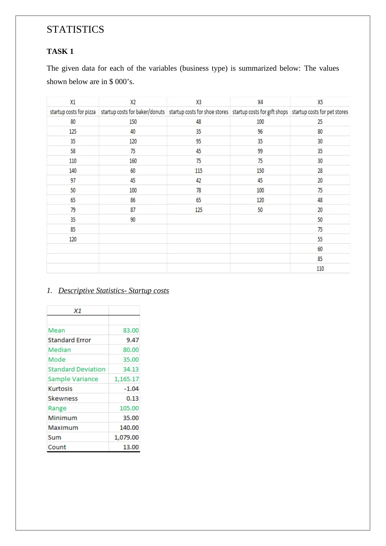
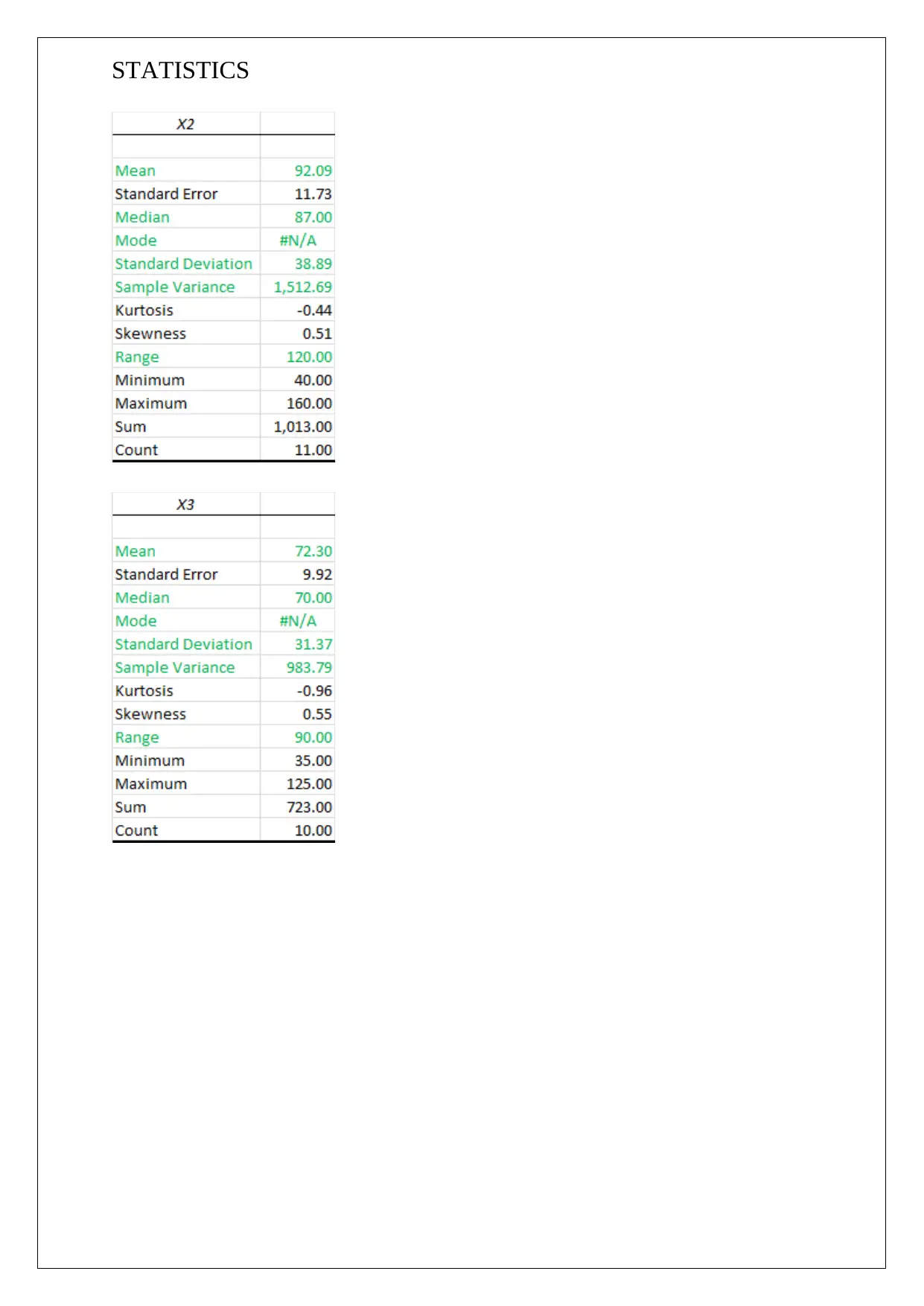
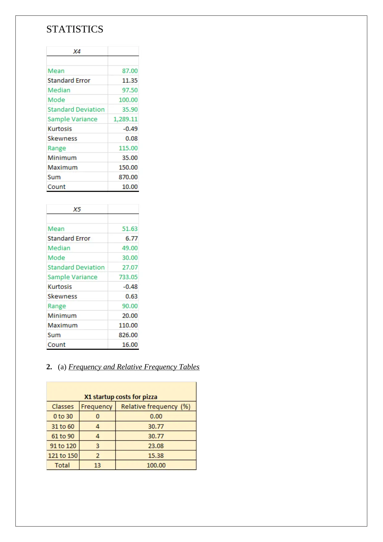
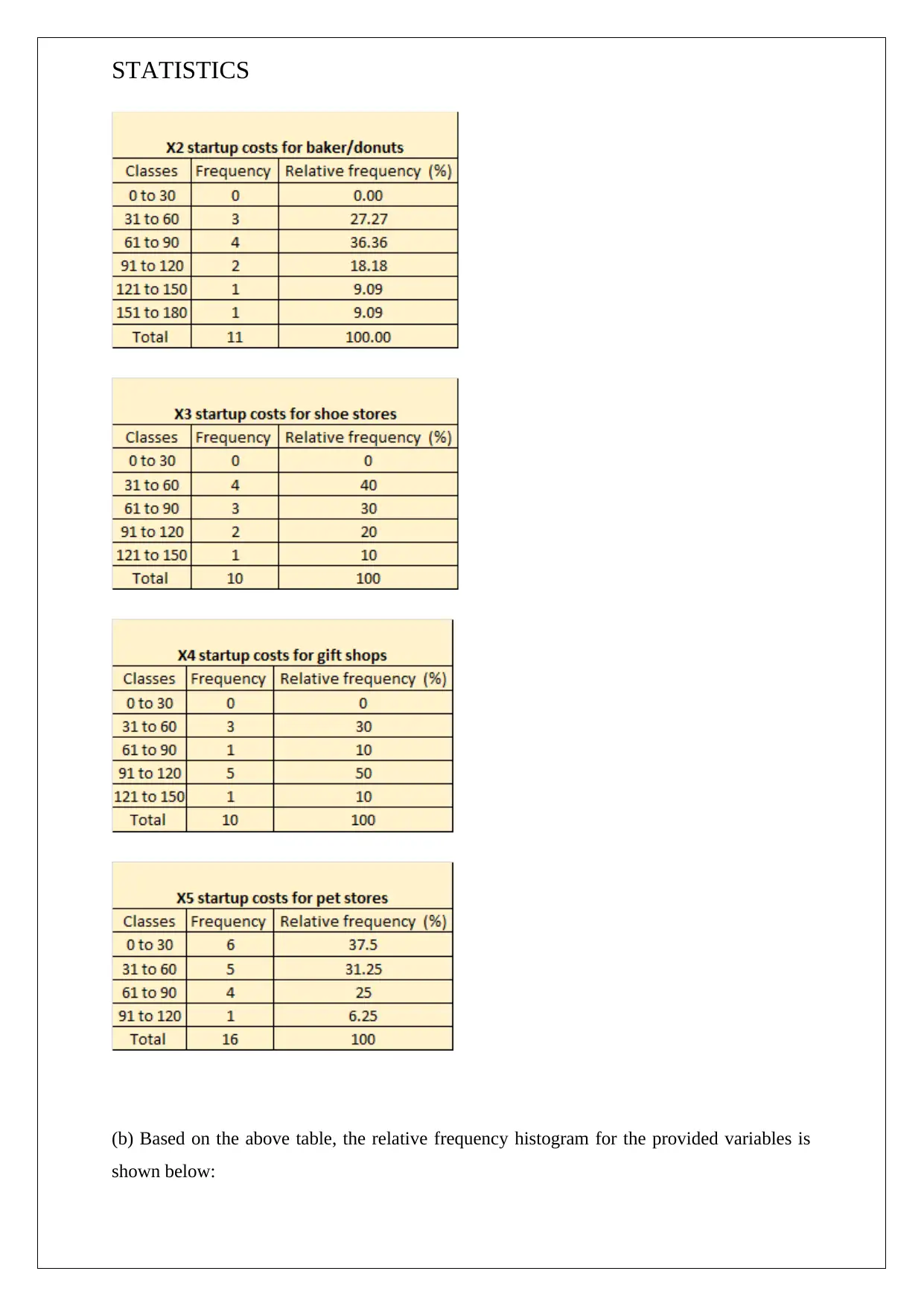
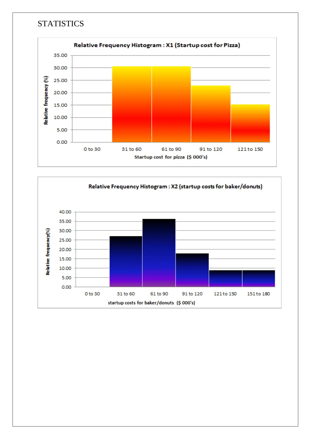
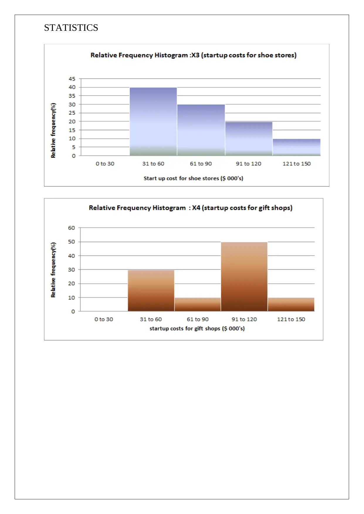
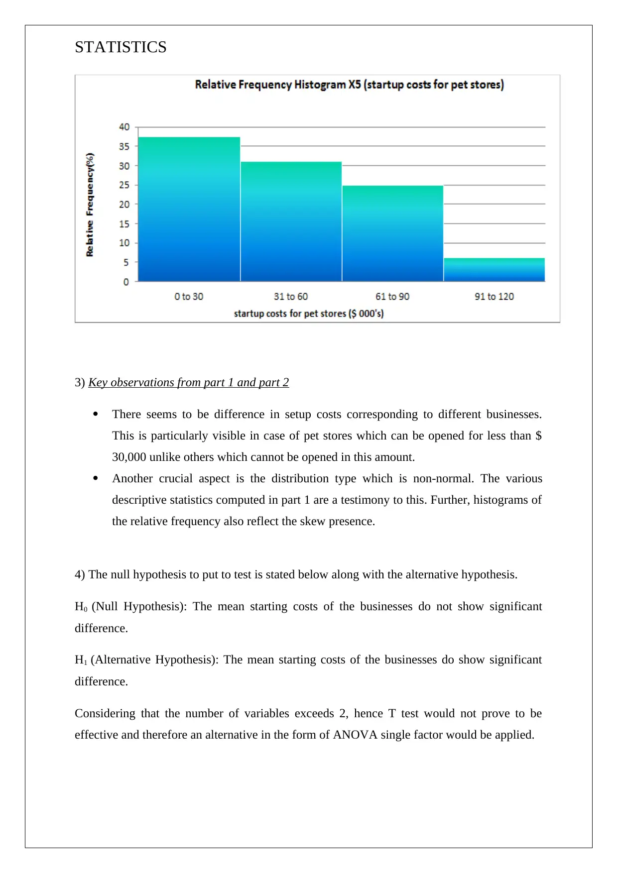
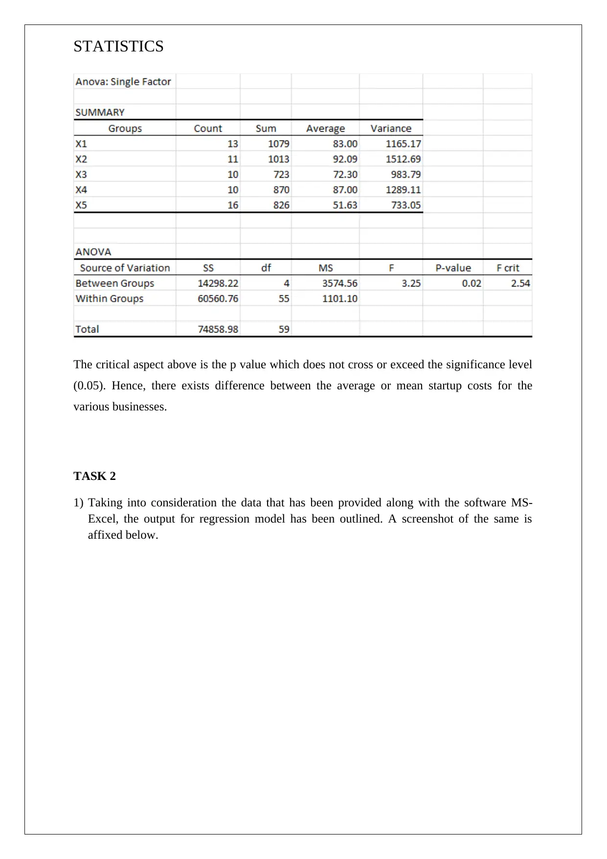
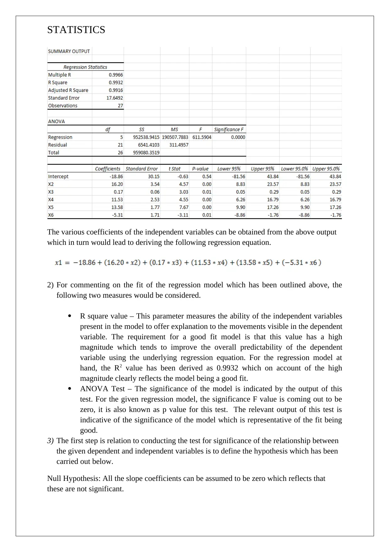
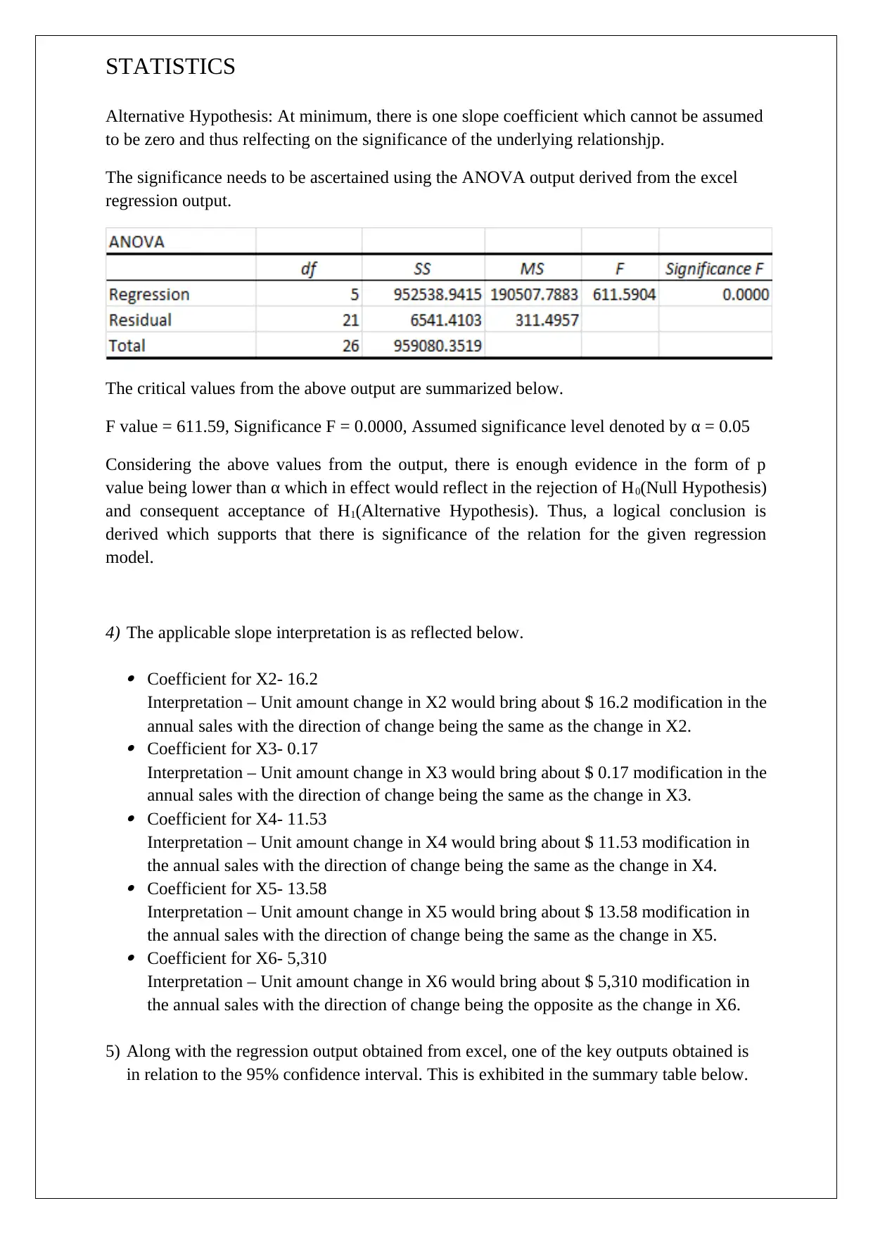
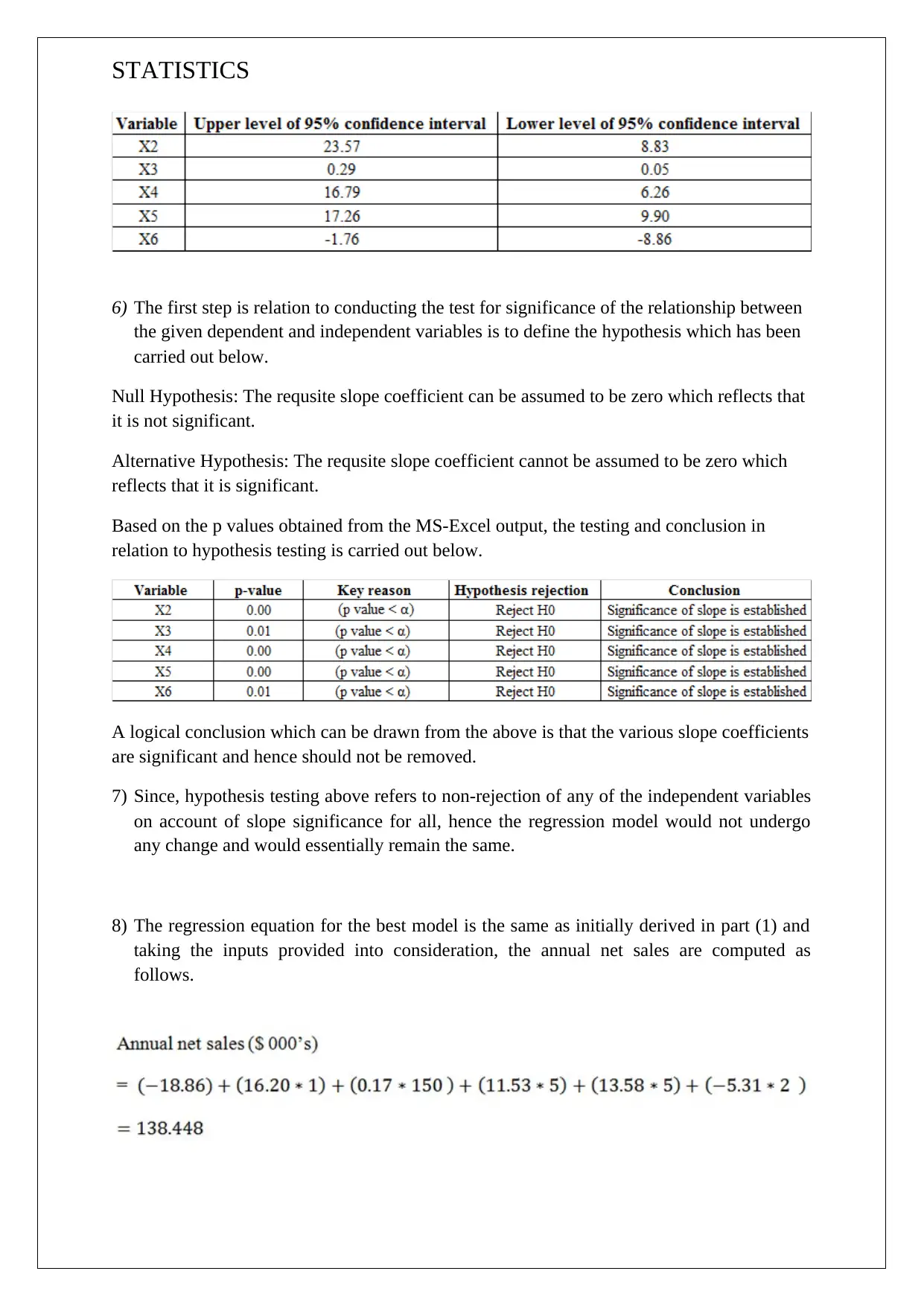
This assignment solution focuses on statistical analysis for business decisions, encompassing two main tasks. Task 1 involves descriptive statistics of startup costs for different business types, including frequency tables, histograms, and key observations regarding cost variations and distribution types. Hypothesis testing using ANOVA is conducted to determine if there are significant differences in mean startup costs. Task 2 delves into regression analysis, using MS-Excel to create a regression model. The solution provides the regression equation, assesses model fit using R-squared and ANOVA tests, and interprets slope coefficients for independent variables. Hypothesis testing is performed to assess the significance of slope coefficients, and the 95% confidence interval is analyzed. The assignment concludes that all slope coefficients are significant, and the regression model remains unchanged, computing annual net sales based on the derived equation.

STATISTICS FOR BUSINESS DECISIONS
STUDENT ID:
[Pick the date]

STATISTICS
TASK 1
The given data for each of the variables (business type) is summarized below: The values
shown below are in $ 000’s.
1. Descriptive Statistics- Startup costs

STATISTICS

STATISTICS
2. (a) Frequency and Relative Frequency Tables

STATISTICS
(b) Based on the above table, the relative frequency histogram for the provided variables is
shown below:

STATISTICS

STATISTICS

STATISTICS
3) Key observations from part 1 and part 2
 There seems to be difference in setup costs corresponding to different businesses.
This is particularly visible in case of pet stores which can be opened for less than $
30,000 unlike others which cannot be opened in this amount.
 Another crucial aspect is the distribution type which is non-normal. The various
descriptive statistics computed in part 1 are a testimony to this. Further, histograms of
the relative frequency also reflect the skew presence.
4) The null hypothesis to put to test is stated below along with the alternative hypothesis.
H0 (Null Hypothesis): The mean starting costs of the businesses do not show significant
difference.
H1 (Alternative Hypothesis): The mean starting costs of the businesses do show significant
difference.
Considering that the number of variables exceeds 2, hence T test would not prove to be
effective and therefore an alternative in the form of ANOVA single factor would be applied.

STATISTICS
The critical aspect above is the p value which does not cross or exceed the significance level
(0.05). Hence, there exists difference between the average or mean startup costs for the
various businesses.
TASK 2
1) Taking into consideration the data that has been provided along with the software MS-
Excel, the output for regression model has been outlined. A screenshot of the same is
affixed below.

STATISTICS
The various coefficients of the independent variables can be obtained from the above output
which in turn would lead to deriving the following regression equation.
2) For commenting on the fit of the regression model which has been outlined above, the
following two measures would be considered.
 R square value – This parameter measures the ability of the independent variables
present in the model to offer explanation to the movements visible in the dependent
variable. The requirement for a good fit model is that this value has a high
magnitude which tends to improve the overall predictability of the dependent
variable using the underlying regression equation. For the regression model at
hand, the R2 value has been derived as 0.9932 which on account of the high
magnitude clearly reflects the model being a good fit.
 ANOVA Test – The significance of the model is indicated by the output of this
test. For the given regression model, the significance F value is coming out to be
zero, it is also known as p value for this test. The relevant output of this test is
indicative of the significance of the model which is representative of the fit being
good.
3) The first step is relation to conducting the test for significance of the relationship between
the given dependent and independent variables is to define the hypothesis which has been
carried out below.
Null Hypothesis: All the slope coefficients can be assumed to be zero which reflects that
these are not significant.

STATISTICS
Alternative Hypothesis: At minimum, there is one slope coefficient which cannot be assumed
to be zero and thus relfecting on the significance of the underlying relationshjp.
The significance needs to be ascertained using the ANOVA output derived from the excel
regression output.
The critical values from the above output are summarized below.
F value = 611.59, Significance F = 0.0000, Assumed significance level denoted by α = 0.05
Considering the above values from the output, there is enough evidence in the form of p
value being lower than α which in effect would reflect in the rejection of H0(Null Hypothesis)
and consequent acceptance of H1(Alternative Hypothesis). Thus, a logical conclusion is
derived which supports that there is significance of the relation for the given regression
model.
4) The applicable slope interpretation is as reflected below.
 Coefficient for X2- 16.2
Interpretation – Unit amount change in X2 would bring about $ 16.2 modification in the
annual sales with the direction of change being the same as the change in X2.
 Coefficient for X3- 0.17
Interpretation – Unit amount change in X3 would bring about $ 0.17 modification in the
annual sales with the direction of change being the same as the change in X3.
 Coefficient for X4- 11.53
Interpretation – Unit amount change in X4 would bring about $ 11.53 modification in
the annual sales with the direction of change being the same as the change in X4.
 Coefficient for X5- 13.58
Interpretation – Unit amount change in X5 would bring about $ 13.58 modification in
the annual sales with the direction of change being the same as the change in X5.
 Coefficient for X6- 5,310
Interpretation – Unit amount change in X6 would bring about $ 5,310 modification in
the annual sales with the direction of change being the opposite as the change in X6.
5) Along with the regression output obtained from excel, one of the key outputs obtained is
in relation to the 95% confidence interval. This is exhibited in the summary table below.

STATISTICS
6) The first step is relation to conducting the test for significance of the relationship between
the given dependent and independent variables is to define the hypothesis which has been
carried out below.
Null Hypothesis: The requsite slope coefficient can be assumed to be zero which reflects that
it is not significant.
Alternative Hypothesis: The requsite slope coefficient cannot be assumed to be zero which
reflects that it is significant.
Based on the p values obtained from the MS-Excel output, the testing and conclusion in
relation to hypothesis testing is carried out below.
A logical conclusion which can be drawn from the above is that the various slope coefficients
are significant and hence should not be removed.
7) Since, hypothesis testing above refers to non-rejection of any of the independent variables
on account of slope significance for all, hence the regression model would not undergo
any change and would essentially remain the same.
8) The regression equation for the best model is the same as initially derived in part (1) and
taking the inputs provided into consideration, the annual net sales are computed as
follows.