Statistics 8: Business Data Modelling Assignment Analysis Report

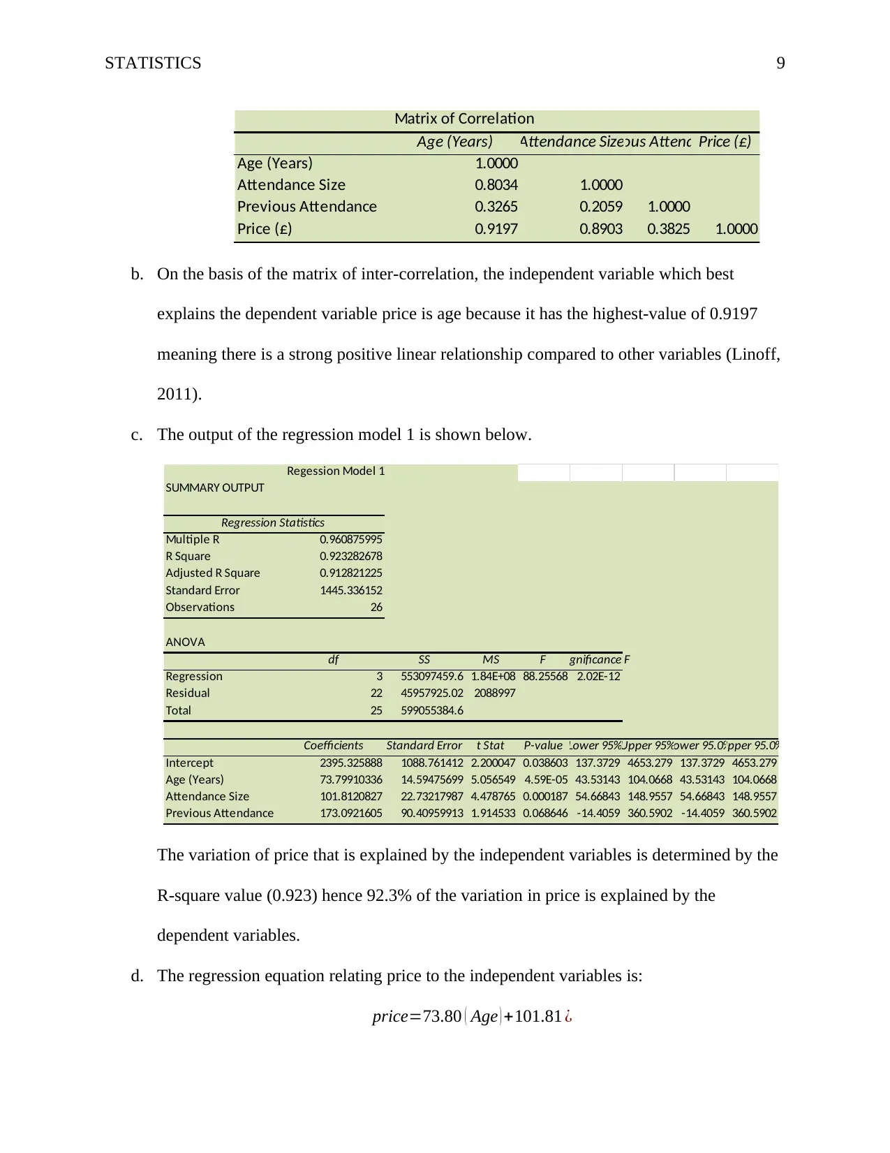
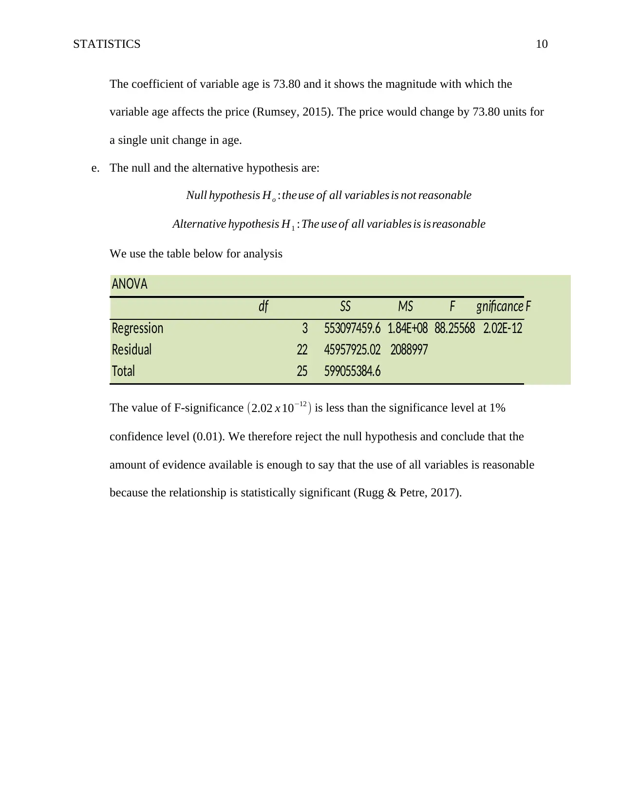
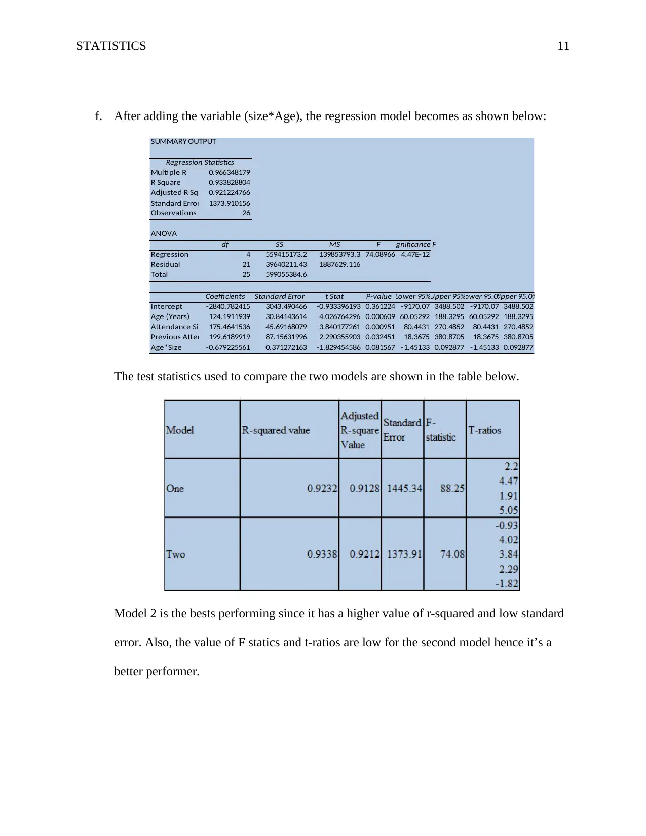
This assignment is a comprehensive analysis of business data modelling using statistical methods. It begins with an examination of categorical variables using a Chi-square test to determine the independence of purchasing behavior and gender. The assignment then proceeds to compare the mean ages of workers at different locations using ANOVA, followed by the Turkey-Kramer test to identify significant mean differences. Finally, it explores relationships between variables such as price, age, and size using scatter plots, correlation matrices, and regression models. The student evaluates the impact of different variables on the regression model's performance, including the addition of interaction variables, and provides interpretations of the results. The assignment includes calculations, interpretations, and critical value comparisons to support conclusions.

Running head: STATISTICS 1
Business Data Modelling
Student Name
Professor’s Name
University Name
Date

STATISTICS 2
Business Data Modelling
Question 1: Analysis of Elect-Mart Company Data
a. Description of Variables
The variable gender is a categorical/qualitative variable with nominal level of
measurement. On the other hand, the variable Buyer Category is a
categorical/qualitative data with ordinal level of measurement.
b. Pivot Table
The pivot table that provides frequency counts for cells created on the basis of variables
gender and buy category is shown below:
c. Testing for independence
To test whether purchasing behavior of customer is related to gender we use the Chi
square test for independence. The test statistic follows the Pearson’s Chi Square
Distribution. The degrees of freedom are given:
df =(R−1)( C−1)
df = ( 3−1 ) ( 2−1 )
df =2
d. Critical Value Approach to Test for Independence.
The null and the alternative hypothesis are stated as follows:
Null hypothesis Ho :Gender∧Buying Category areindependent
Alternative hypothesis H1 :Gender∧Buying category are not independent

STATISTICS 3
The test statistic is given by:
X2 =∑ (O−E)2
E
Where O is the frequency observed, and E the frequency that is expected.
The observed frequencies are shown below:
The expected frequencies are given by:
E= Row total∗column total
N
The are summarized in the table below.
Expected Frequecies
Row High Low Medium Total
Female 62.95 81.60 59.45 204.00
Male 45.05 58.40 42.55 146.00
Total 108.00 140.00 102.00 350.00
The Test Statistics is given by:
X2 =(69.0−62.95)2
62.95 + (79−81.6)2
81.6 + (56−59.45)2
59.45 + (39−45.05)2
45.05 + (61−58.40)2
58.40 +( 46−42.55)2
42.55
X2 =0.58+0.08+0.20+0.81+ 0.12+0.28
X2 =2.07
For 2 degrees of freedom and 0.01 significance level the critical value from the chi-
square table is 9.2104. The decision rule is that we reject the null hypothesis if the test
statistic determined is greater than the critical value. In this case:
Ho : x2 calc< x2 critic

STATISTICS 4
2.07< 9.21
Therefore, we fail to reject the null hypothesis since there is sufficient evidence to prove
that buying category and gender are independent of each other.
Question 2: Hypothesis Test for Mean
a. The methodology that would be used to compare the mean ages of the workers at the four
locations is the analysis of variance. The type of variations that get used in the test are;
Explained variation and Unexplained Variation. The distribution follows the F-test
distribution. The degrees of freedom are given by:
df t =df B +df w
The degrees of freedom between groups is given by the number of groups minus 1:
df B=Ngroups−1
df B=4−1=3
The degrees of freedom within the groups is given by the total number of subjects minus
the number of groups:
df w=N−Ngroups
df w=24−4=20
Total degrees of freedom:
df t =20+3=23 degrees of freedom
b. The null and the alternative hypothesis are stated as below:
The null hypothesis is that there is no difference in the means while the alternative
hypothesis is that at least one of the means is different.
Null hypothesis Ho : μ1=μ2 ¿ μ3 ¿ μ4
Alternative Hypothesis H1 : μ1 ≠ μ2 ≠ μ3 ≠ μ4

STATISTICS 5
The Group mean is given by:
GM =( μ1 +μ2 + μ3 + μ4
Ngroups )
GM =( 28.71+32.5+24.8+26.83
4 )=28.21
We assess the variability between and within the groups.
The variability between groups is determined by the sum of squares between groups
given by:
SSB=n1 ( μ1−GM ) 2 +n2 ( μ2−GM )
2+ n3 ( μ3−GM ) 2+n4 ( μ4 −GM ) 2
SSB=7 ( 0.25 ) + 6 ( 18.40 ) + 5 ( 11.63 ) +6 (1.90)
SSB=181.70
The variability within the groups is given by the sum of the squares within groups:
SSW =SS 1+ SS 2+SS 3+ SS 4
The values of sum of squares “SS” are determined in the excel sheet.
SSW = ( 13.43+17.5+2.8+ 54.83 )=88.56
The total sum of squares is:
SST =SSB+SSW
SST =181.70+ 88.56=270.26
The ratio of the sum of the squares to the degrees of freedom obtained previously is:
The means square between groups:
MSB= SSB
df b
= 181.70
3 =60.57
The mean square within groups:
MSW = SSW
df w
= 88.56
20 =4.428

STATISTICS 6
The F-statistic is the ratio of the mean square between to mean square within and is given
by:
F statistic= MSB
MSW =60.57
4.428 =13.68
The ANOVA table can be created as follows
The Critical value of F from the degrees of freedom at 5% significance level on the F-
table is 3.098. The decision rule is that we reject the null hypothesis if the test statistic is
greater than the critical value. In this case 13.63>3.098 therefore we reject the null
hypothesis and conclude that enough evidence is available to prove that at least one of the
means is different.
c. Determination of which mean is different
We use the Turkey-Kramer test. The output is developed in excel and is as shown below.
TUKEY HSD/KRAMER alpha 0.05
group mean n ss df q-crit
A 28.71 7.00 13.43
B 32.50 6.00 17.50
C 24.80 5.00 2.80
D 26.83 6.00 54.83
24.00 88.56 20.00 3.96
Q TEST
group 1 group 2 mean std err q-stat lower upper p-value mean-crit Cohen d
A B 3.79 0.83 4.57 0.51 7.06 0.02 3.28 1.80
A C 3.91 0.87 4.49 0.47 7.36 0.02 3.45 1.86
A D 1.88 0.83 2.27 -1.40 5.16 0.40 3.28 0.89
B C 7.70 0.90 8.55 4.13 11.27 0.00 3.57 3.66
B D 5.67 0.86 6.60 2.27 9.07 0.00 3.40 2.69
C D 2.03 0.90 2.26 -1.53 5.60 0.40 3.57 0.97
By comparing the P-values of the combinations at 5% significance level, we see that the
only significant combinations are AB, AC, BC, and BD (Lock, 2013). The combinations

STATISTICS 7
AD and CD are not significant and therefore there is a difference in mean between the
pairs A and D and the pairs C and D.
Question 3
a. Scatter Plots and Matrix of inter-correlations
I. Price and Age
The relationship between price and age is a strong positive linear relationship.
II. Price and Size
The relationship between price and size is a moderately strong positive linear
relationship.
III. Price and Previous Attendance

STATISTICS 8
The relationship between price and attendance is a weak positive linear
relationship.
IV. Size and Age
The relationship between age and size is a moderately strong positive linear
relationship.
The relationships make sense because price is likely to increase with increase in
previous attendance, the age and the attendance size. Also, the attendance size is
expected to increase with age.
The matrix of the intercorrelation between the variables is shown in the table
below.

STATISTICS 9
Matrix of Correlation
Age (Years) Attendance SizePrevious AttendancePrice (£)
Age (Years) 1.0000
Attendance Size 0.8034 1.0000
Previous Attendance 0.3265 0.2059 1.0000
Price (£) 0.9197 0.8903 0.3825 1.0000
b. On the basis of the matrix of inter-correlation, the independent variable which best
explains the dependent variable price is age because it has the highest-value of 0.9197
meaning there is a strong positive linear relationship compared to other variables (Linoff,
2011).
c. The output of the regression model 1 is shown below.
Regession Model 1
SUMMARY OUTPUT
Regression Statistics
Multiple R 0.960875995
R Square 0.923282678
Adjusted R Square 0.912821225
Standard Error 1445.336152
Observations 26
ANOVA
df SS MS F Significance F
Regression 3 553097459.6 1.84E+08 88.25568 2.02E-12
Residual 22 45957925.02 2088997
Total 25 599055384.6
Coefficients Standard Error t Stat P-value Lower 95%Upper 95%Lower 95.0%Upper 95.0%
Intercept 2395.325888 1088.761412 2.200047 0.038603 137.3729 4653.279 137.3729 4653.279
Age (Years) 73.79910336 14.59475699 5.056549 4.59E-05 43.53143 104.0668 43.53143 104.0668
Attendance Size 101.8120827 22.73217987 4.478765 0.000187 54.66843 148.9557 54.66843 148.9557
Previous Attendance 173.0921605 90.40959913 1.914533 0.068646 -14.4059 360.5902 -14.4059 360.5902
The variation of price that is explained by the independent variables is determined by the
R-square value (0.923) hence 92.3% of the variation in price is explained by the
dependent variables.
d. The regression equation relating price to the independent variables is:
price=73.80 ( Age ) +101.81 ¿

STATISTICS 10
The coefficient of variable age is 73.80 and it shows the magnitude with which the
variable age affects the price (Rumsey, 2015). The price would change by 73.80 units for
a single unit change in age.
e. The null and the alternative hypothesis are:
Null hypothesis Ho :theuse of all variables is not reasonable
Alternative hypothesis H1 :The use of all variables is isreasonable
We use the table below for analysis
ANOVA
df SS MS F Significance F
Regression 3 553097459.6 1.84E+08 88.25568 2.02E-12
Residual 22 45957925.02 2088997
Total 25 599055384.6
The value of F-significance (2.02 x 10−12 ) is less than the significance level at 1%
confidence level (0.01). We therefore reject the null hypothesis and conclude that the
amount of evidence available is enough to say that the use of all variables is reasonable
because the relationship is statistically significant (Rugg & Petre, 2017).

STATISTICS 11
f. After adding the variable (size*Age), the regression model becomes as shown below:
SUMMARY OUTPUT
Regression Statistics
Multiple R 0.966348179
R Square 0.933828804
Adjusted R Square0.921224766
Standard Error 1373.910156
Observations 26
ANOVA
df SS MS F Significance F
Regression 4 559415173.2 139853793.3 74.08966 4.47E-12
Residual 21 39640211.43 1887629.116
Total 25 599055384.6
Coefficients Standard Error t Stat P-value Lower 95%Upper 95%Lower 95.0%Upper 95.0%
Intercept -2840.782415 3043.490466 -0.933396193 0.361224 -9170.07 3488.502 -9170.07 3488.502
Age (Years) 124.1911939 30.84143614 4.026764296 0.000609 60.05292 188.3295 60.05292 188.3295
Attendance Size 175.4641536 45.69168079 3.840177261 0.000951 80.4431 270.4852 80.4431 270.4852
Previous Attendance199.6189919 87.15631996 2.290355903 0.032451 18.3675 380.8705 18.3675 380.8705
Age*Size -0.679225561 0.371272163 -1.829454586 0.081567 -1.45133 0.092877 -1.45133 0.092877
The test statistics used to compare the two models are shown in the table below.
Model 2 is the bests performing since it has a higher value of r-squared and low standard
error. Also, the value of F statics and t-ratios are low for the second model hence it’s a
better performer.

STATISTICS 12
g. The variable (age*size) is an integration variable that is added to the model to increase
the performance of the model. Yes, it is reasonable to use the variable in the model since
improved the prediction capability of the regression model.
h. The inclusion of the variable age*size in the regression model only increases the R-
square values and adjusted R-square values and not the t-ratios because the integration
variables only meant to increase the prediction ability of the model and not its precision.
With increased prediction capability, the precision would come down and that is why the
t-ratios are not significant.
i. The regression equation for the second equation is:
price=124.19 ( Age ) +175.46 ¿
Hence the prediction is:
price=124.9 ( 90 )+175.46 ( 110 )+199.61 ( 8 ) −0.679 ( 9900 ) +2840.78
Price=28193.36
The standard error is 1373.91. and the critical value of t at 95% confidence level and 25
degrees of freedom is 2.06. Therefore, the margin of error is:
Me=se∗t value
me=1373.91 x 2.06
me=2830.25
There the 95% prediction interval for the price would be:
25363.11 ≤ p ≤31023.61
References

STATISTICS 13
Linoff, G. (2011). Data analysis using SQL and Excel. Indianapolis, Ind.: Wiley Pub.
Lock, R. (2013). Statistics: Unlocking the power of data. Wiley.
Rugg, G., & Petre, M. (2017). A gentle guide to research methods. Maidenhead: Open
University Press.
Rumsey, D. (2015). Intermediate statistics for dummies (1st ed). Hoboken, N.J.: Wiley.