Statistics for Management: Evaluating Business Data and Planning
VerifiedAdded on 2021/02/21
|21
|4225
|34
Report
AI Summary
This report, titled "Statistics for Management," presents a detailed analysis of business and economic data using various statistical methods. The report begins with an introduction that highlights the importance of statistics in modern business decision-making. Task 1 evaluates business and economic data from diverse published sources, employing t-distribution to compare mean earnings between men and women in both public and private sectors, and calculating annual growth rates. Task 2 focuses on analyzing and evaluating qualitative and quantitative raw business data, including the use of scatter plots to determine the association between hot drink sales and average temperature, calculating correlation coefficients and coefficients of determination, and determining the line of best fit for sales predictions. The report concludes with an evaluation of the reliability of these predictions and factors that may impact the sales values. The report provides comprehensive insights into data analysis and its applications in business planning for quality, inventory, and capacity management.
STATISTICS FOR
MANAGEMENT
MANAGEMENT
Paraphrase This Document
Need a fresh take? Get an instant paraphrase of this document with our AI Paraphraser
Table of Contents
INTRODUCTION...........................................................................................................................1
TASK 1............................................................................................................................................1
P1. Evaluating the nature and process of business and economic data/ information from a
range of different published sources............................................................................................1
P2. Business Data from variety of sources using different methods of analysis.........................3
TASK 2............................................................................................................................................4
P3. Analysing and evaluating qualitative and quantitative raw business data using appropriate
statistical methods........................................................................................................................4
TASK 3............................................................................................................................................8
P4. Application of a range of statistical methods used in business planning for quality,
inventory and capacity management............................................................................................8
TASK 4..........................................................................................................................................11
P5. Utilisation of appropriate charts/ tables to communicate findings for a number of given
variables.....................................................................................................................................11
CONCLUSION..............................................................................................................................13
REFERENCES..............................................................................................................................14
APPENDICES...............................................................................................................................15
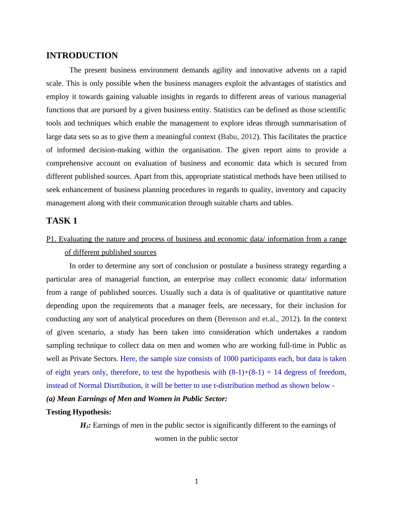
INTRODUCTION
The present business environment demands agility and innovative advents on a rapid
scale. This is only possible when the business managers exploit the advantages of statistics and
employ it towards gaining valuable insights in regards to different areas of various managerial
functions that are pursued by a given business entity. Statistics can be defined as those scientific
tools and techniques which enable the management to explore ideas through summarisation of
large data sets so as to give them a meaningful context (Babu, 2012). This facilitates the practice
of informed decision-making within the organisation. The given report aims to provide a
comprehensive account on evaluation of business and economic data which is secured from
different published sources. Apart from this, appropriate statistical methods have been utilised to
seek enhancement of business planning procedures in regards to quality, inventory and capacity
management along with their communication through suitable charts and tables.
TASK 1
P1. Evaluating the nature and process of business and economic data/ information from a range
of different published sources
In order to determine any sort of conclusion or postulate a business strategy regarding a
particular area of managerial function, an enterprise may collect economic data/ information
from a range of published sources. Usually such a data is of qualitative or quantitative nature
depending upon the requirements that a manager feels, are necessary, for their inclusion for
conducting any sort of analytical procedures on them (Berenson and et.al., 2012). In the context
of given scenario, a study has been taken into consideration which undertakes a random
sampling technique to collect data on men and women who are working full-time in Public as
well as Private Sectors. Here, the sample size consists of 1000 participants each, but data is taken
of eight years only, therefore, to test the hypothesis with (8-1)+(8-1) = 14 degress of freedom,
instead of Normal Disrtibution, it will be better to use t-distribution method as shown below -
(a) Mean Earnings of Men and Women in Public Sector:
Testing Hypothesis:
H1: Earnings of men in the public sector is significantly different to the earnings of
women in the public sector
1
⊘ This is a preview!⊘
Do you want full access?
Subscribe today to unlock all pages.
Trusted by 1+ million students worldwide
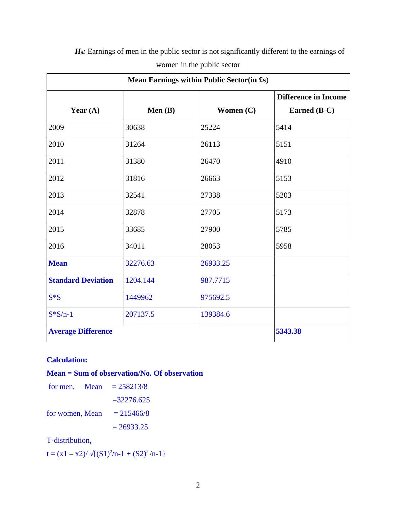
H0: Earnings of men in the public sector is not significantly different to the earnings of
women in the public sector
Mean Earnings within Public Sector(in £s)
Year (A) Men (B) Women (C)
Difference in Income
Earned (B-C)
2009 30638 25224 5414
2010 31264 26113 5151
2011 31380 26470 4910
2012 31816 26663 5153
2013 32541 27338 5203
2014 32878 27705 5173
2015 33685 27900 5785
2016 34011 28053 5958
Mean 32276.63 26933.25
Standard Deviation 1204.144 987.7715
S*S 1449962 975692.5
S*S/n-1 207137.5 139384.6
Average Difference 5343.38
Calculation:
Mean = Sum of observation/No. Of observation
for men, Mean = 258213/8
=32276.625
for women, Mean = 215466/8
= 26933.25
T-distribution,
t = (x1 – x2)/ √[(S1)2/n-1 + (S2)2 /n-1}
2
Paraphrase This Document
Need a fresh take? Get an instant paraphrase of this document with our AI Paraphraser
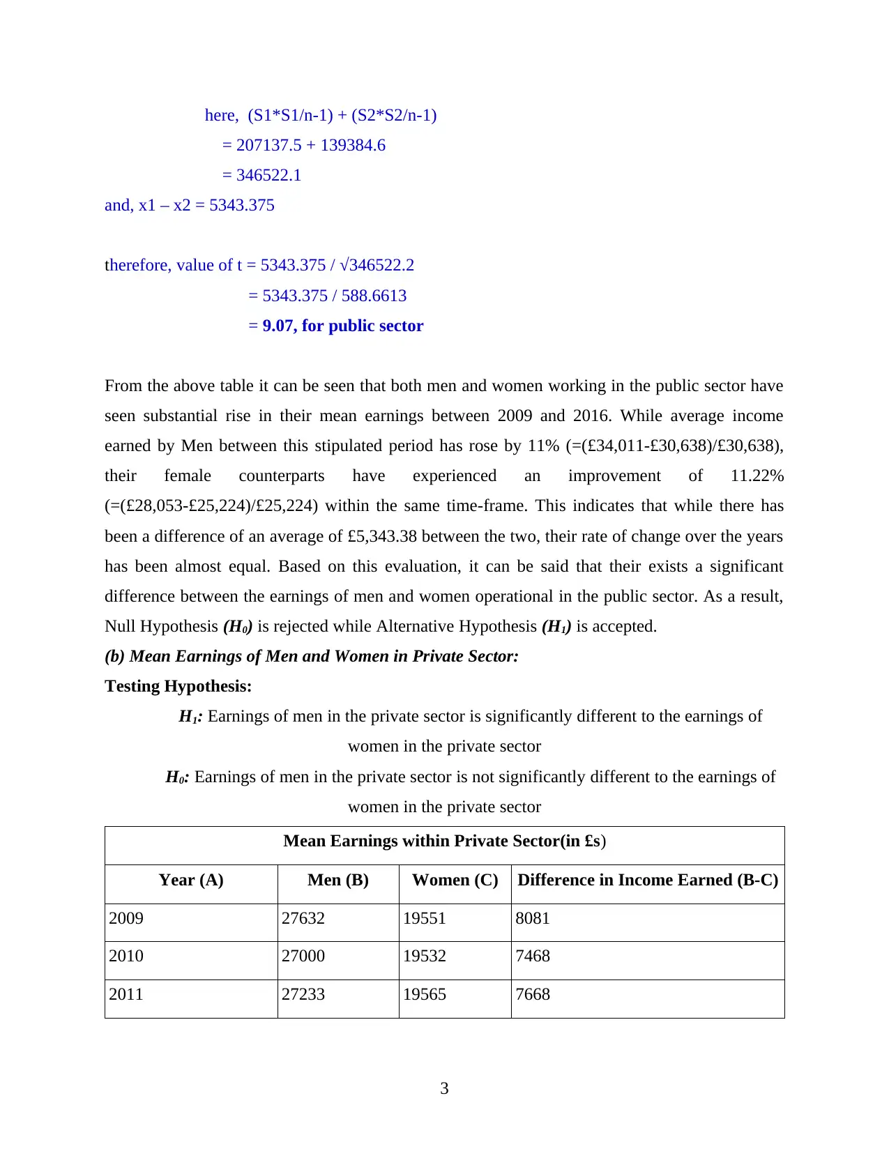
here, (S1*S1/n-1) + (S2*S2/n-1)
= 207137.5 + 139384.6
= 346522.1
and, x1 – x2 = 5343.375
therefore, value of t = 5343.375 / √346522.2
= 5343.375 / 588.6613
= 9.07, for public sector
From the above table it can be seen that both men and women working in the public sector have
seen substantial rise in their mean earnings between 2009 and 2016. While average income
earned by Men between this stipulated period has rose by 11% (=(£34,011-£30,638)/£30,638),
their female counterparts have experienced an improvement of 11.22%
(=(£28,053-£25,224)/£25,224) within the same time-frame. This indicates that while there has
been a difference of an average of £5,343.38 between the two, their rate of change over the years
has been almost equal. Based on this evaluation, it can be said that their exists a significant
difference between the earnings of men and women operational in the public sector. As a result,
Null Hypothesis (H0) is rejected while Alternative Hypothesis (H1) is accepted.
(b) Mean Earnings of Men and Women in Private Sector:
Testing Hypothesis:
H1: Earnings of men in the private sector is significantly different to the earnings of
women in the private sector
H0: Earnings of men in the private sector is not significantly different to the earnings of
women in the private sector
Mean Earnings within Private Sector(in £s)
Year (A) Men (B) Women (C) Difference in Income Earned (B-C)
2009 27632 19551 8081
2010 27000 19532 7468
2011 27233 19565 7668
3
2012 27705 20313 7392
2013 28201 20698 7503
2014 28442 21017 7425
2015 28881 21403 7478
2016 29679 22251 7428
Mean 28096.53 20541.25
Standard Deviation 834.1923 994.349
S*S 695876.7 988729.9
S*S/n-1 99410.96 141247.1
Average Difference 7555.38
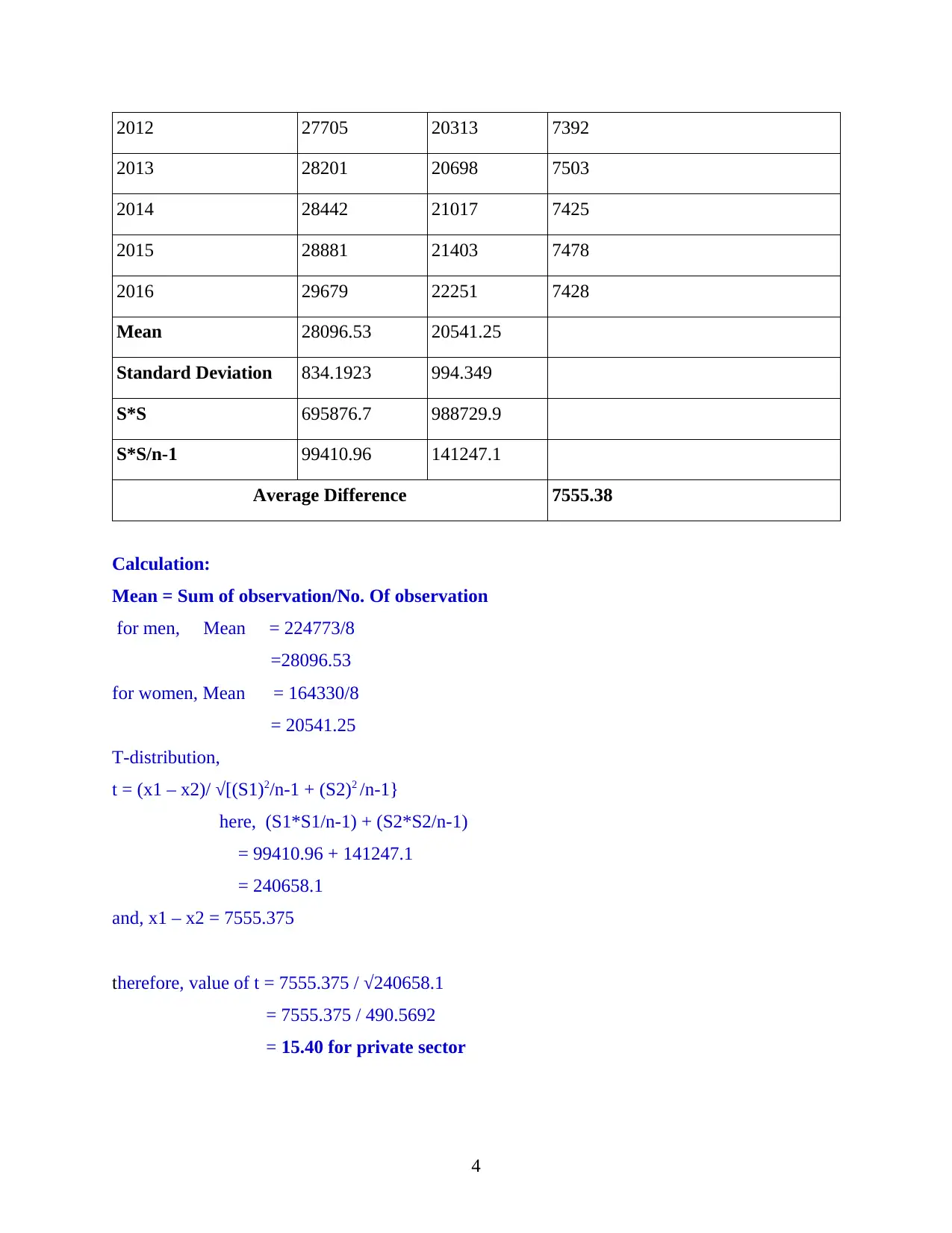
Calculation:
Mean = Sum of observation/No. Of observation
for men, Mean = 224773/8
=28096.53
for women, Mean = 164330/8
= 20541.25
T-distribution,
t = (x1 – x2)/ √[(S1)2/n-1 + (S2)2 /n-1}
here, (S1*S1/n-1) + (S2*S2/n-1)
= 99410.96 + 141247.1
= 240658.1
and, x1 – x2 = 7555.375
therefore, value of t = 7555.375 / √240658.1
= 7555.375 / 490.5692
= 15.40 for private sector
4
2013 28201 20698 7503
2014 28442 21017 7425
2015 28881 21403 7478
2016 29679 22251 7428
Mean 28096.53 20541.25
Standard Deviation 834.1923 994.349
S*S 695876.7 988729.9
S*S/n-1 99410.96 141247.1
Average Difference 7555.38
Calculation:
Mean = Sum of observation/No. Of observation
for men, Mean = 224773/8
=28096.53
for women, Mean = 164330/8
= 20541.25
T-distribution,
t = (x1 – x2)/ √[(S1)2/n-1 + (S2)2 /n-1}
here, (S1*S1/n-1) + (S2*S2/n-1)
= 99410.96 + 141247.1
= 240658.1
and, x1 – x2 = 7555.375
therefore, value of t = 7555.375 / √240658.1
= 7555.375 / 490.5692
= 15.40 for private sector
4
⊘ This is a preview!⊘
Do you want full access?
Subscribe today to unlock all pages.
Trusted by 1+ million students worldwide
From the above table it is clearly evident that men and women working full time in the Private
Sector have seen a considerable rise over the years. Between 2009 and 2016, mean earnings for
men have increased by 7.41% (=(£29,679-£27,632)/£27,632) whereas for women it is attributed
to be 13.81% (=(£22,251-£19,551)/£19,551). Based on these figures it can be said that the
women working in the private sector have been thriving even more than their male counterparts.
Therefore, based on this evaluation, it can be said that their exists a significant difference
between the earnings of men and women operational in the private sector. As a result, Null
Hypothesis (H0) is rejected while Alternative Hypothesis (H1) is accepted.
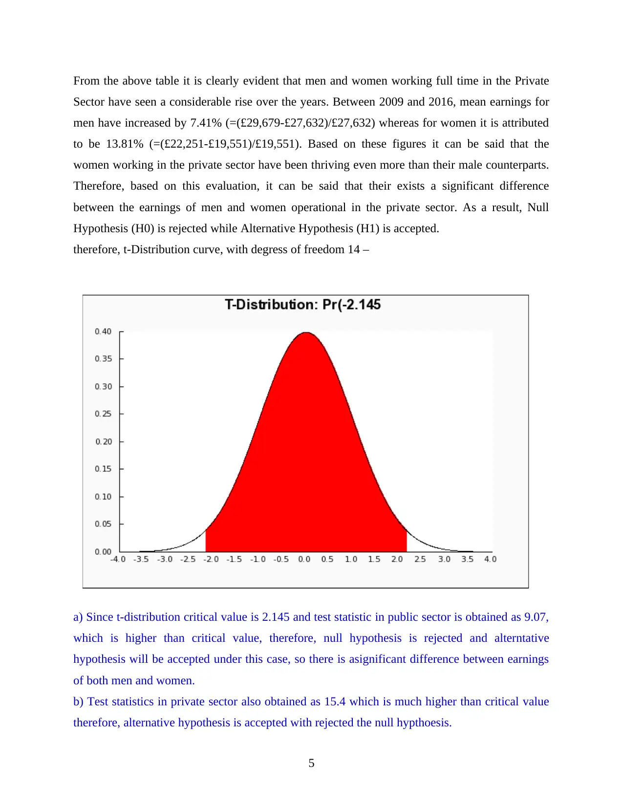
therefore, t-Distribution curve, with degress of freedom 14 –
a) Since t-distribution critical value is 2.145 and test statistic in public sector is obtained as 9.07,
which is higher than critical value, therefore, null hypothesis is rejected and alterntative
hypothesis will be accepted under this case, so there is asignificant difference between earnings
of both men and women.
b) Test statistics in private sector also obtained as 15.4 which is much higher than critical value
therefore, alternative hypothesis is accepted with rejected the null hypthoesis.
5
Sector have seen a considerable rise over the years. Between 2009 and 2016, mean earnings for
men have increased by 7.41% (=(£29,679-£27,632)/£27,632) whereas for women it is attributed
to be 13.81% (=(£22,251-£19,551)/£19,551). Based on these figures it can be said that the
women working in the private sector have been thriving even more than their male counterparts.
Therefore, based on this evaluation, it can be said that their exists a significant difference
between the earnings of men and women operational in the private sector. As a result, Null
Hypothesis (H0) is rejected while Alternative Hypothesis (H1) is accepted.
therefore, t-Distribution curve, with degress of freedom 14 –
a) Since t-distribution critical value is 2.145 and test statistic in public sector is obtained as 9.07,
which is higher than critical value, therefore, null hypothesis is rejected and alterntative
hypothesis will be accepted under this case, so there is asignificant difference between earnings
of both men and women.
b) Test statistics in private sector also obtained as 15.4 which is much higher than critical value
therefore, alternative hypothesis is accepted with rejected the null hypthoesis.
5
Paraphrase This Document
Need a fresh take? Get an instant paraphrase of this document with our AI Paraphraser
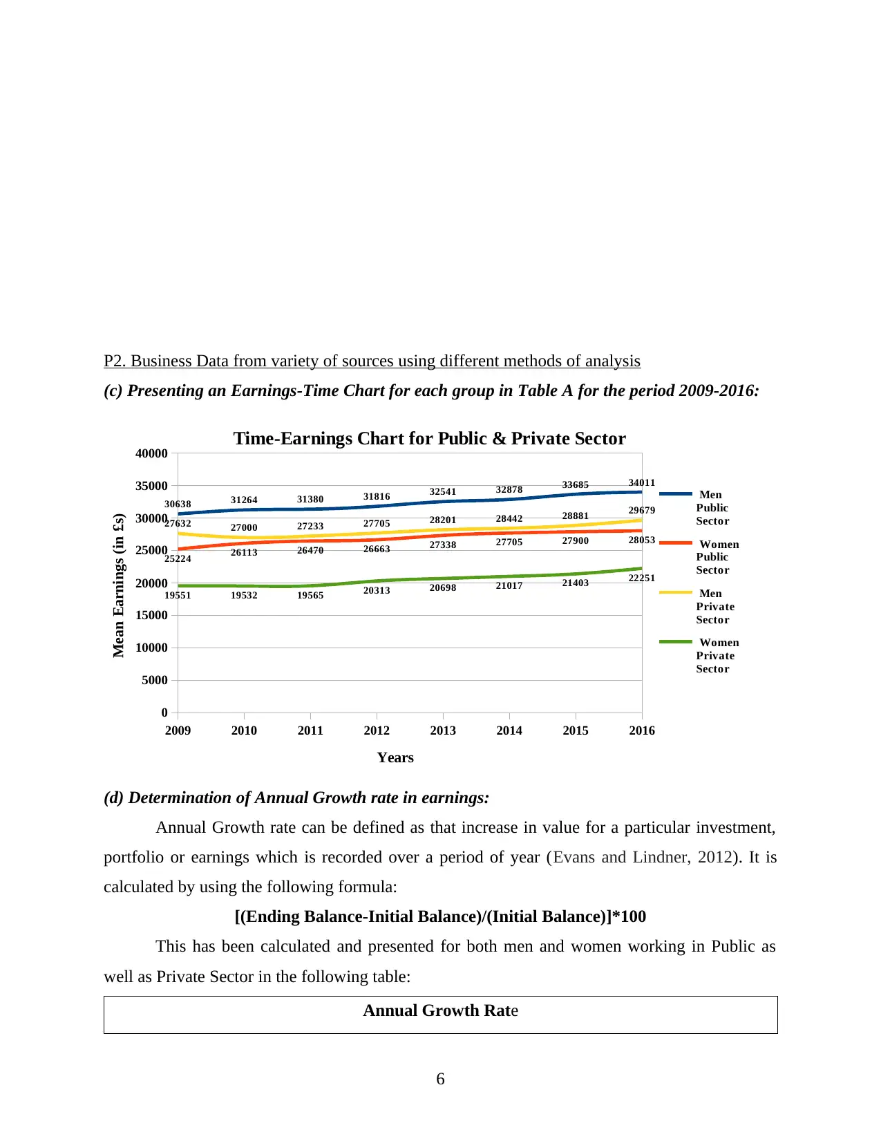
P2. Business Data from variety of sources using different methods of analysis
(c) Presenting an Earnings-Time Chart for each group in Table A for the period 2009-2016:
2009 2010 2011 2012 2013 2014 2015 2016
0
5000
10000
15000
20000
25000
30000
35000
40000
30638 31264 31380 31816 32541 32878 33685 34011
25224 26113 26470 26663 27338 27705 27900 28053
27632 27000 27233 27705 28201 28442 28881 29679
19551 19532 19565 20313 20698 21017 21403 22251
Time-Earnings Chart for Public & Private Sector
Men
Public
Sector
Women
Public
Sector
Men
Private
Sector
Women
Private
Sector
Years
Mean Earnings (in £s)
(d) Determination of Annual Growth rate in earnings:
Annual Growth rate can be defined as that increase in value for a particular investment,
portfolio or earnings which is recorded over a period of year (Evans and Lindner, 2012). It is
calculated by using the following formula:
[(Ending Balance-Initial Balance)/(Initial Balance)]*100
This has been calculated and presented for both men and women working in Public as
well as Private Sector in the following table:
Annual Growth Rate
6
Public Sector Private Sector
Year Men Women Men Women
2009 0.00% 0.00% 0.00% 0.00%
2010 2.04% 3.52% -2.29% -0.10%
2011 0.37% 1.37% 0.86% 0.17%
2012 1.39% 0.73% 1.73% 3.82%
2013 2.28% 2.53% 1.79% 1.90%
2014 1.04% 1.34% 0.85% 1.54%
2015 2.45% 0.70% 1.54% 1.84%
2016 0.97% 0.55% 2.76% 3.96%
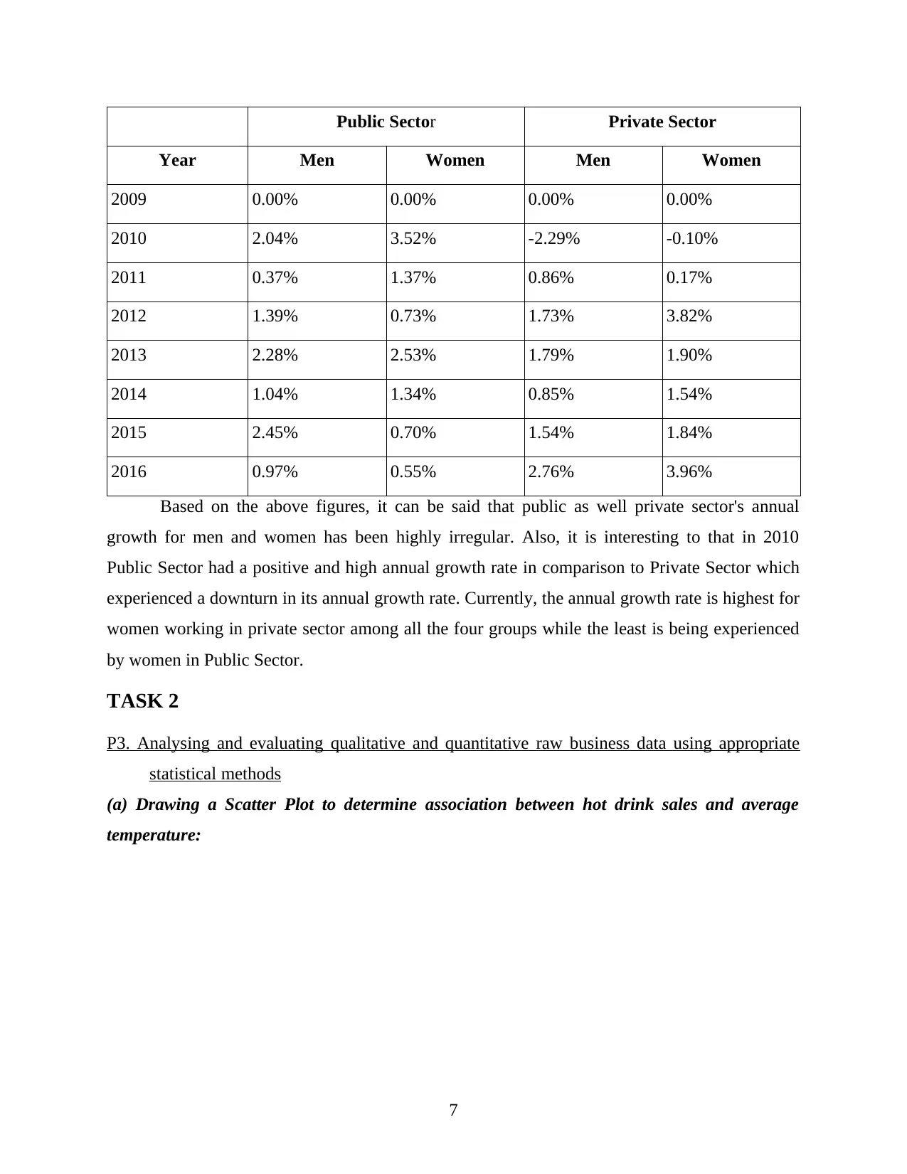
Based on the above figures, it can be said that public as well private sector's annual
growth for men and women has been highly irregular. Also, it is interesting to that in 2010
Public Sector had a positive and high annual growth rate in comparison to Private Sector which
experienced a downturn in its annual growth rate. Currently, the annual growth rate is highest for
women working in private sector among all the four groups while the least is being experienced
by women in Public Sector.
TASK 2
P3. Analysing and evaluating qualitative and quantitative raw business data using appropriate
statistical methods
(a) Drawing a Scatter Plot to determine association between hot drink sales and average
temperature:
7
Year Men Women Men Women
2009 0.00% 0.00% 0.00% 0.00%
2010 2.04% 3.52% -2.29% -0.10%
2011 0.37% 1.37% 0.86% 0.17%
2012 1.39% 0.73% 1.73% 3.82%
2013 2.28% 2.53% 1.79% 1.90%
2014 1.04% 1.34% 0.85% 1.54%
2015 2.45% 0.70% 1.54% 1.84%
2016 0.97% 0.55% 2.76% 3.96%
Based on the above figures, it can be said that public as well private sector's annual
growth for men and women has been highly irregular. Also, it is interesting to that in 2010
Public Sector had a positive and high annual growth rate in comparison to Private Sector which
experienced a downturn in its annual growth rate. Currently, the annual growth rate is highest for
women working in private sector among all the four groups while the least is being experienced
by women in Public Sector.
TASK 2
P3. Analysing and evaluating qualitative and quantitative raw business data using appropriate
statistical methods
(a) Drawing a Scatter Plot to determine association between hot drink sales and average
temperature:
7
⊘ This is a preview!⊘
Do you want full access?
Subscribe today to unlock all pages.
Trusted by 1+ million students worldwide
12 13 14 15 16 17 18 19 20 21
0
2
4
6
8
10
12
14
16
18
20
15
10
13.5
15
18
14
13
8.5
6
9
Scatter Plot
Hot Drink Sales
(000s)
Average Temperature (in Celsius)
Hot Drink Sales (in 000s)
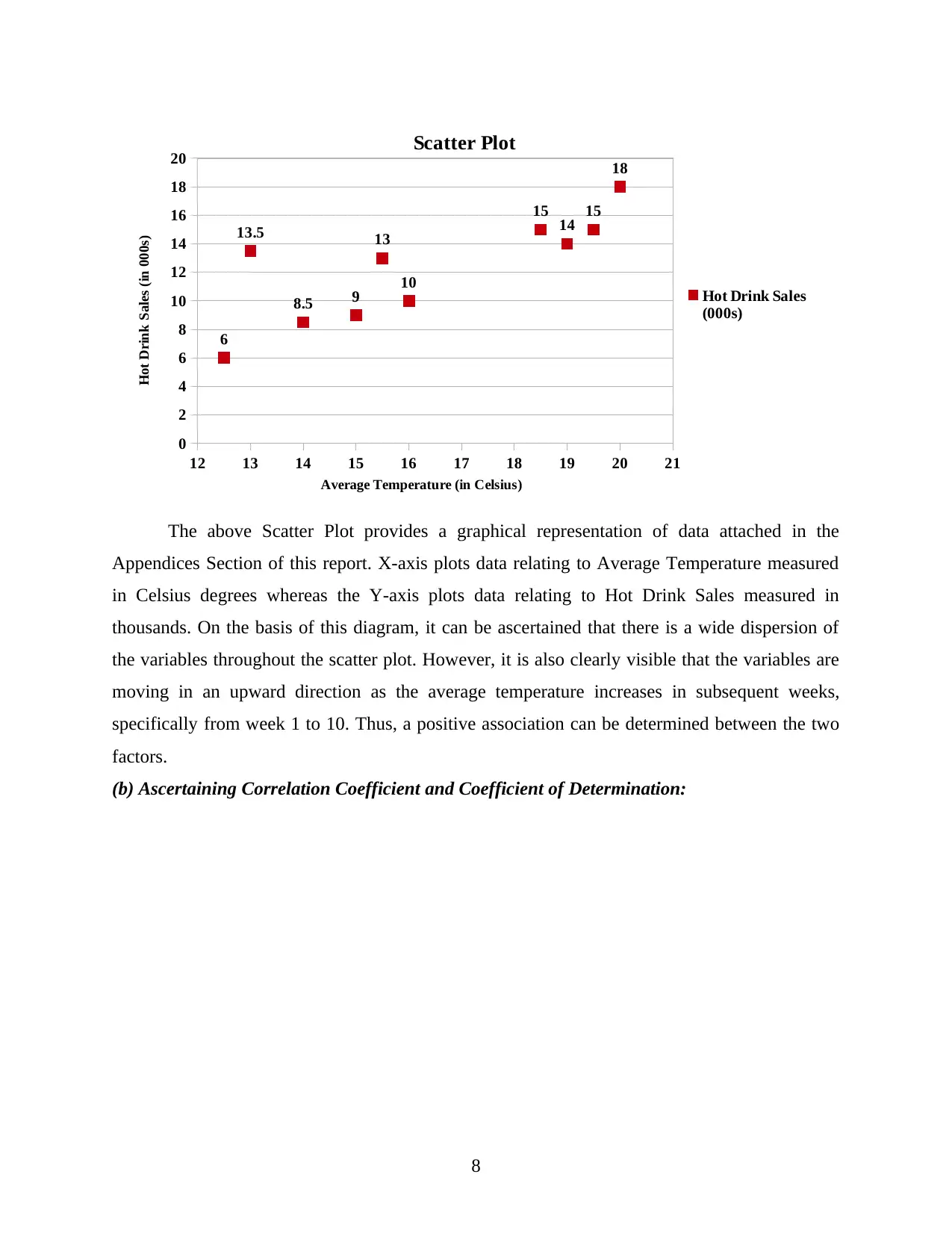
The above Scatter Plot provides a graphical representation of data attached in the
Appendices Section of this report. X-axis plots data relating to Average Temperature measured
in Celsius degrees whereas the Y-axis plots data relating to Hot Drink Sales measured in
thousands. On the basis of this diagram, it can be ascertained that there is a wide dispersion of
the variables throughout the scatter plot. However, it is also clearly visible that the variables are
moving in an upward direction as the average temperature increases in subsequent weeks,
specifically from week 1 to 10. Thus, a positive association can be determined between the two
factors.
(b) Ascertaining Correlation Coefficient and Coefficient of Determination:
8
0
2
4
6
8
10
12
14
16
18
20
15
10
13.5
15
18
14
13
8.5
6
9
Scatter Plot
Hot Drink Sales
(000s)
Average Temperature (in Celsius)
Hot Drink Sales (in 000s)
The above Scatter Plot provides a graphical representation of data attached in the
Appendices Section of this report. X-axis plots data relating to Average Temperature measured
in Celsius degrees whereas the Y-axis plots data relating to Hot Drink Sales measured in
thousands. On the basis of this diagram, it can be ascertained that there is a wide dispersion of
the variables throughout the scatter plot. However, it is also clearly visible that the variables are
moving in an upward direction as the average temperature increases in subsequent weeks,
specifically from week 1 to 10. Thus, a positive association can be determined between the two
factors.
(b) Ascertaining Correlation Coefficient and Coefficient of Determination:
8
Paraphrase This Document
Need a fresh take? Get an instant paraphrase of this document with our AI Paraphraser
12 13 14 15 16 17 18 19 20 21
0
2
4
6
8
10
12
14
16
18
20
15
10
13.5
15
18
14
13
8.5
6
9
f(x) = 1.06222865412446 x − 5.11432706222865
R² = 0.638555145067446
Scatter Plot
Hot Drink
Sales (000s)
Linear (Hot
Drink Sales
(000s))
Average Temperature (in Celsius)
Hot Drink Sales (in 000s)
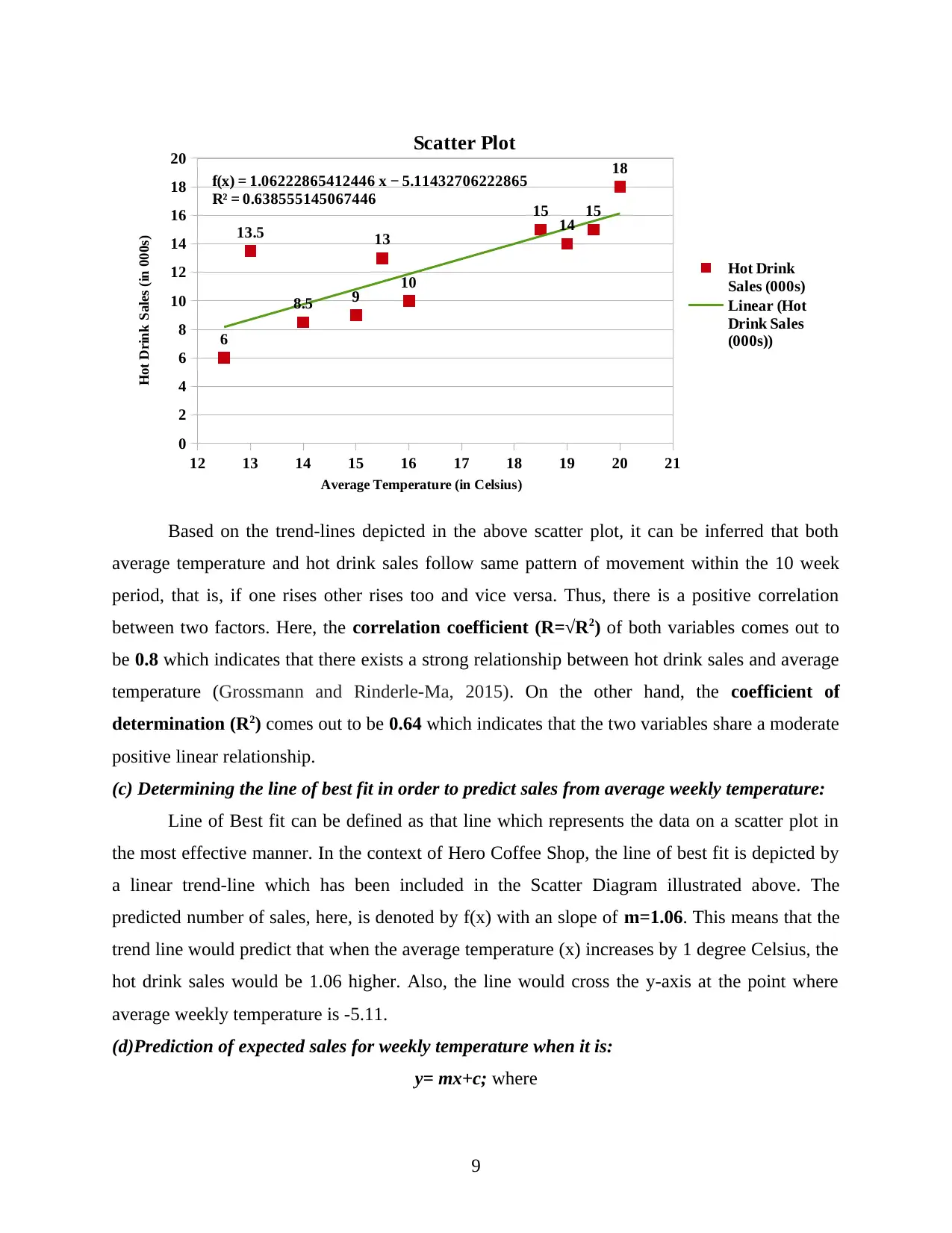
Based on the trend-lines depicted in the above scatter plot, it can be inferred that both
average temperature and hot drink sales follow same pattern of movement within the 10 week
period, that is, if one rises other rises too and vice versa. Thus, there is a positive correlation
between two factors. Here, the correlation coefficient (R=√R2) of both variables comes out to
be 0.8 which indicates that there exists a strong relationship between hot drink sales and average
temperature (Grossmann and Rinderle-Ma, 2015). On the other hand, the coefficient of
determination (R2) comes out to be 0.64 which indicates that the two variables share a moderate
positive linear relationship.
(c) Determining the line of best fit in order to predict sales from average weekly temperature:
Line of Best fit can be defined as that line which represents the data on a scatter plot in
the most effective manner. In the context of Hero Coffee Shop, the line of best fit is depicted by
a linear trend-line which has been included in the Scatter Diagram illustrated above. The
predicted number of sales, here, is denoted by f(x) with an slope of m=1.06. This means that the
trend line would predict that when the average temperature (x) increases by 1 degree Celsius, the
hot drink sales would be 1.06 higher. Also, the line would cross the y-axis at the point where
average weekly temperature is -5.11.
(d)Prediction of expected sales for weekly temperature when it is:
y= mx+c; where
9
0
2
4
6
8
10
12
14
16
18
20
15
10
13.5
15
18
14
13
8.5
6
9
f(x) = 1.06222865412446 x − 5.11432706222865
R² = 0.638555145067446
Scatter Plot
Hot Drink
Sales (000s)
Linear (Hot
Drink Sales
(000s))
Average Temperature (in Celsius)
Hot Drink Sales (in 000s)
Based on the trend-lines depicted in the above scatter plot, it can be inferred that both
average temperature and hot drink sales follow same pattern of movement within the 10 week
period, that is, if one rises other rises too and vice versa. Thus, there is a positive correlation
between two factors. Here, the correlation coefficient (R=√R2) of both variables comes out to
be 0.8 which indicates that there exists a strong relationship between hot drink sales and average
temperature (Grossmann and Rinderle-Ma, 2015). On the other hand, the coefficient of
determination (R2) comes out to be 0.64 which indicates that the two variables share a moderate
positive linear relationship.
(c) Determining the line of best fit in order to predict sales from average weekly temperature:
Line of Best fit can be defined as that line which represents the data on a scatter plot in
the most effective manner. In the context of Hero Coffee Shop, the line of best fit is depicted by
a linear trend-line which has been included in the Scatter Diagram illustrated above. The
predicted number of sales, here, is denoted by f(x) with an slope of m=1.06. This means that the
trend line would predict that when the average temperature (x) increases by 1 degree Celsius, the
hot drink sales would be 1.06 higher. Also, the line would cross the y-axis at the point where
average weekly temperature is -5.11.
(d)Prediction of expected sales for weekly temperature when it is:
y= mx+c; where
9
y= function of x
m= slope of the equation
c= intercept
(i) 17.5 degree Celsius:
In this case, the predicted expected sales (in 000s) of Hero Coffee Shop are calculated as under:
y = mx+c
y=1.06x-5.11
y=[(1.06*17.5)-5.11]
y=[(18.55)-(5.11)]
y=13.44 or 13,440 units of hot drinks
(ii)25 degree Celsius:
In this case, the predicted expected sales (in 000s) of Hero Coffee Shop are calculated as under:
y = mx+c
y=1.06x-5.11
y=[(1.06*25)-5.11]
y=[(26.50)-(5.11)]
y=21.39 or 21,390 units of hot drinks
(e) Evaluating the reliability of predictions made in regards to additional factors which may
impact the sales values achieved:
The reliability of predictions made in regards to the expected sales of Hero Coffee Shop's
hot drinks in association with the average weekly temperature is not high. This is due to the fact
that there are other additional factors which may impact the sales values achieved in the Task 2.
P3. Part (d)(i) and (ii) sections of this report. Some of them include the shop's budget, its
efficiency in catering to the customer demand as well as ensuing competition in the external
environment among others (Groebner and et.al., 2013). Thus, it can be concluded that although
there is a considerable amount of impact on hot drink sales due to temperature, accounting it as
the sole reason for making predictions on the sale of such products is not highly reliable.
10
⊘ This is a preview!⊘
Do you want full access?
Subscribe today to unlock all pages.
Trusted by 1+ million students worldwide
1 out of 21
Related Documents


Your All-in-One AI-Powered Toolkit for Academic Success.
+13062052269
info@desklib.com
Available 24*7 on WhatsApp / Email
![[object Object]](/_next/static/media/star-bottom.7253800d.svg)
Unlock your academic potential
Copyright © 2020–2026 A2Z Services. All Rights Reserved. Developed and managed by ZUCOL.