BUS5SBF Assignment: Statistical Analysis of Household Data and Finance

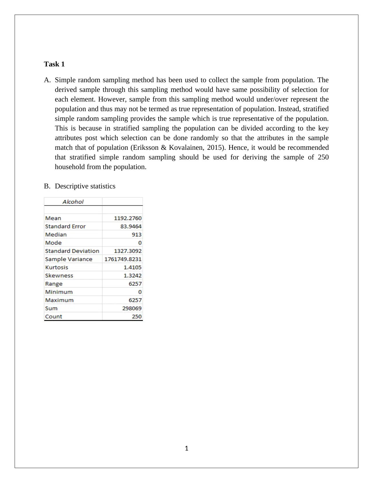
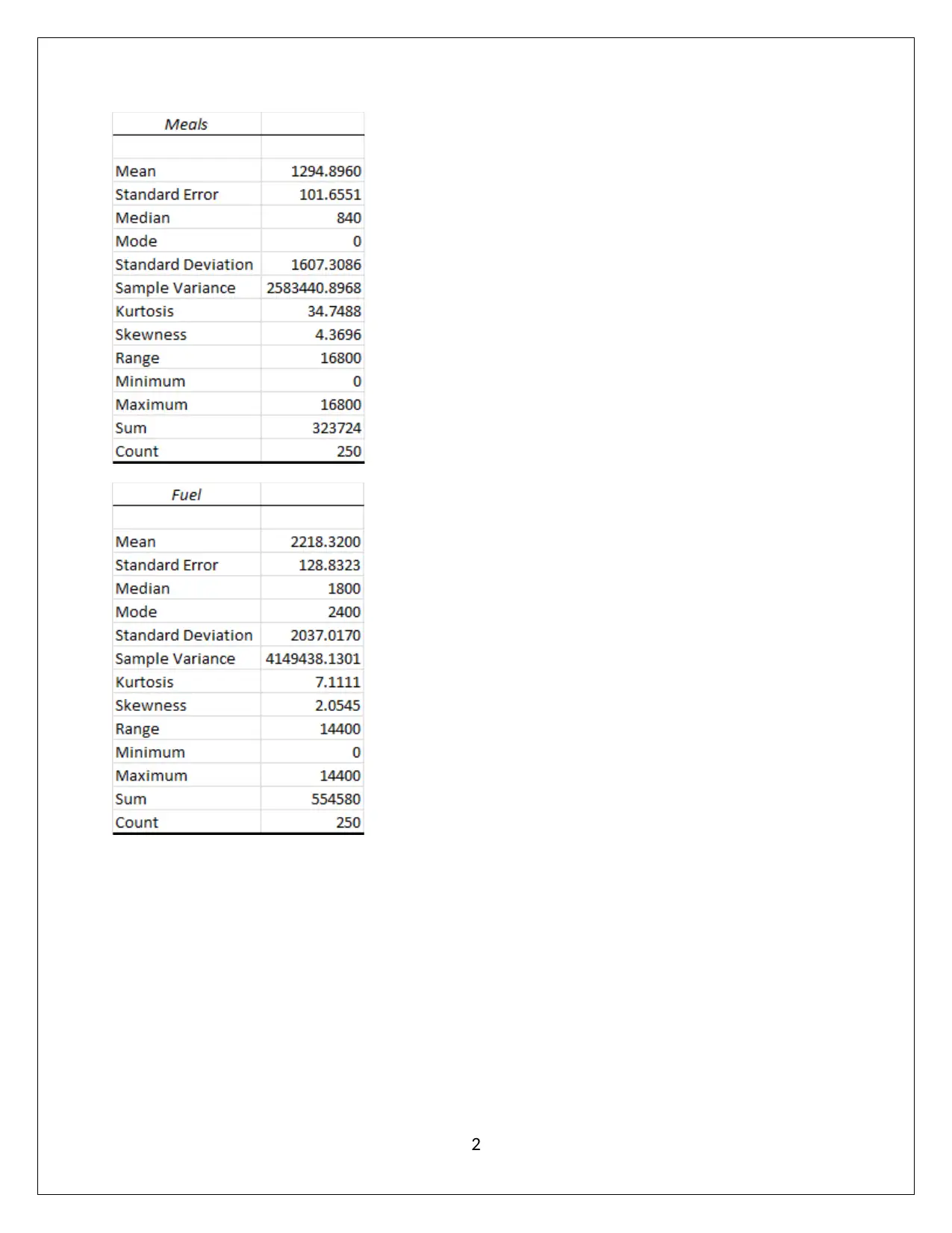
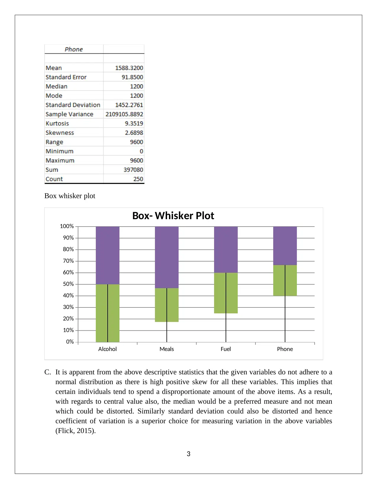
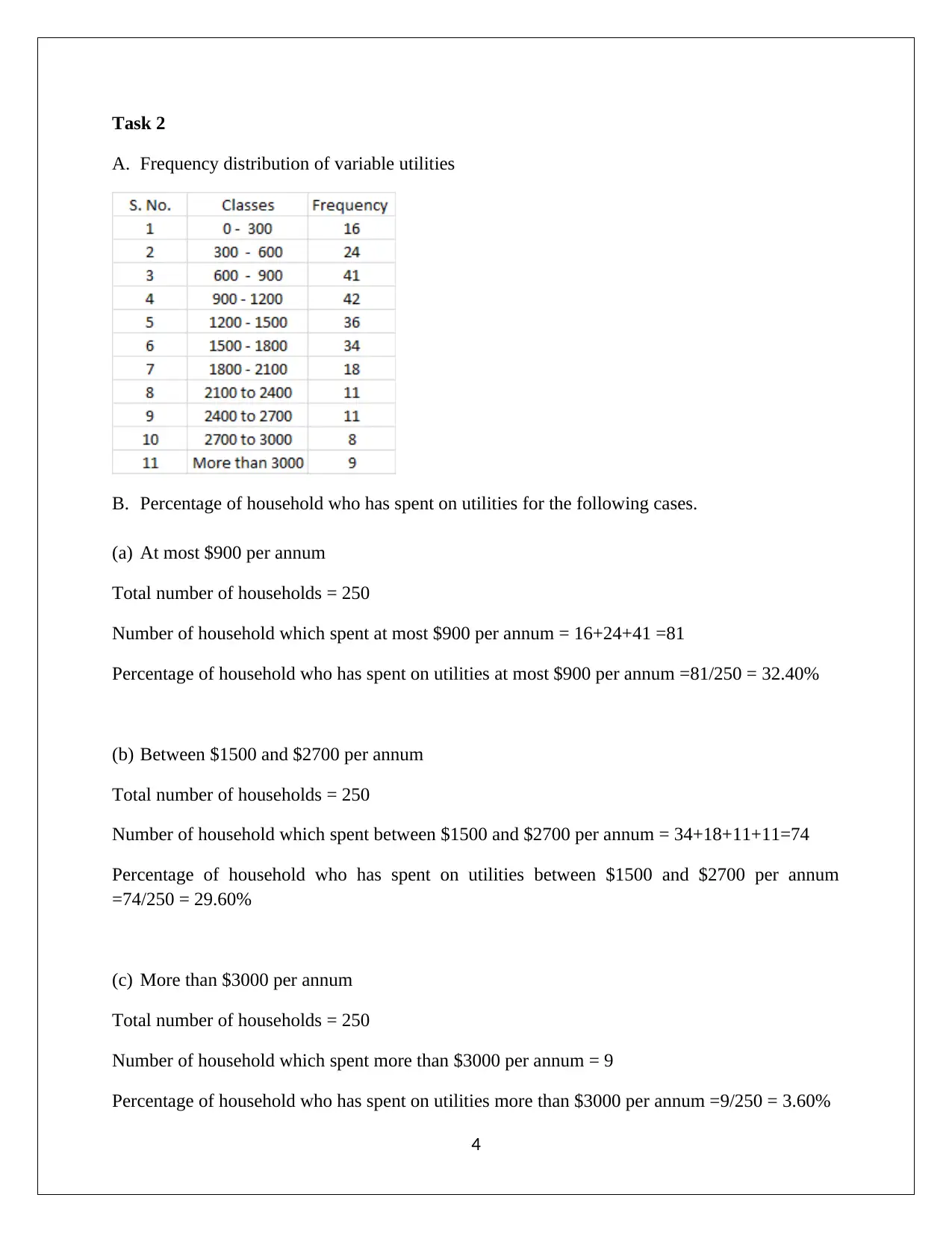
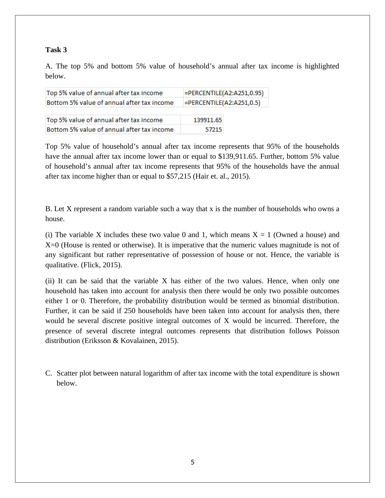
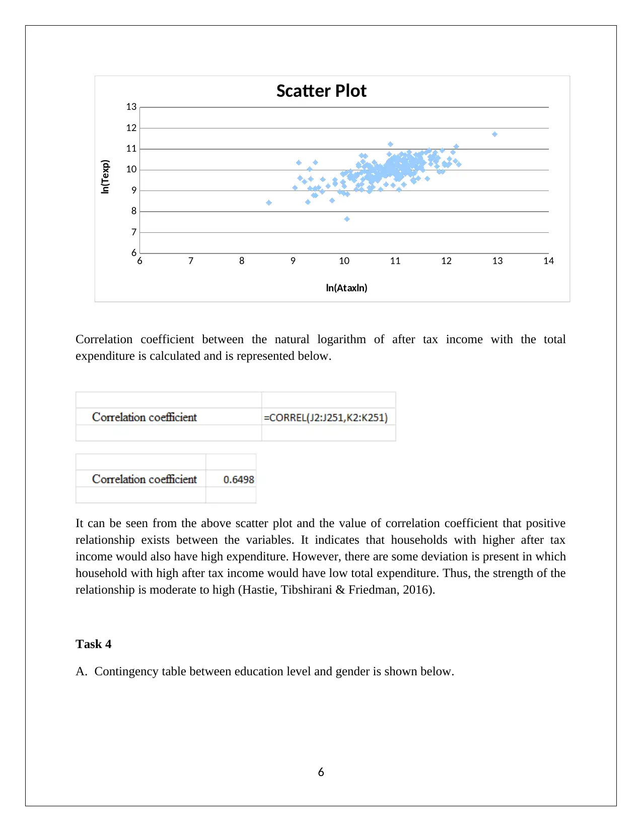
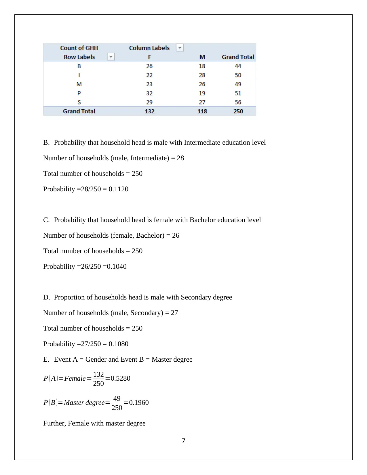
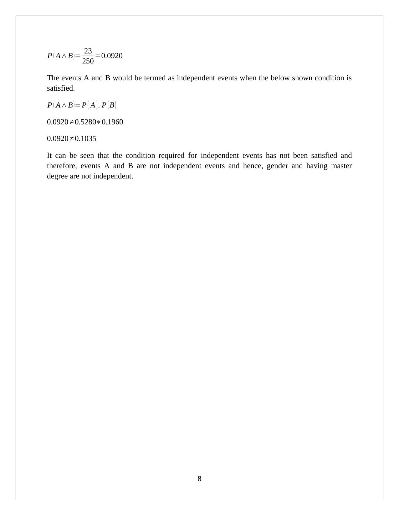
This assignment analyzes household data using statistical methods for a Business and Finance course. It begins with a discussion of sampling methods, recommending stratified simple random sampling. The solution then presents descriptive statistics using box-whisker plots and discusses the skewness of the data, suggesting the use of the median and coefficient of variation. The assignment continues with frequency distributions, calculating percentages for utility spending. Further, the analysis covers the top and bottom 5% of after-tax income, discusses the nature of variables (qualitative vs. quantitative), and explores probability distributions. The solution also includes a scatter plot and correlation analysis between after-tax income and total expenditure. Finally, it presents a contingency table analyzing the relationship between education level and gender, calculating probabilities and assessing the independence of events.

Statistics For Business and Finance
Analyzing Household Data
Student Name
[Pick the date]

Task 1
A. Simple random sampling method has been used to collect the sample from population. The
derived sample through this sampling method would have same possibility of selection for
each element. However, sample from this sampling method would under/over represent the
population and thus may not be termed as true representation of population. Instead, stratified
simple random sampling provides the sample which is true representative of the population.
This is because in stratified sampling the population can be divided according to the key
attributes post which selection can be done randomly so that the attributes in the sample
match that of population (Eriksson & Kovalainen, 2015). Hence, it would be recommended
that stratified simple random sampling should be used for deriving the sample of 250
household from the population.
B. Descriptive statistics
1

2

Box whisker plot
Alcohol Meals Fuel Phone
0%
10%
20%
30%
40%
50%
60%
70%
80%
90%
100%
Box- Whisker Plot
C. It is apparent from the above descriptive statistics that the given variables do not adhere to a
normal distribution as there is high positive skew for all these variables. This implies that
certain individuals tend to spend a disproportionate amount of the above items. As a result,
with regards to central value also, the median would be a preferred measure and not mean
which could be distorted. Similarly standard deviation could also be distorted and hence
coefficient of variation is a superior choice for measuring variation in the above variables
(Flick, 2015).
3

Task 2
A. Frequency distribution of variable utilities
B. Percentage of household who has spent on utilities for the following cases.
(a) At most $900 per annum
Total number of households = 250
Number of household which spent at most $900 per annum = 16+24+41 =81
Percentage of household who has spent on utilities at most $900 per annum =81/250 = 32.40%
(b) Between $1500 and $2700 per annum
Total number of households = 250
Number of household which spent between $1500 and $2700 per annum = 34+18+11+11=74
Percentage of household who has spent on utilities between $1500 and $2700 per annum
=74/250 = 29.60%
(c) More than $3000 per annum
Total number of households = 250
Number of household which spent more than $3000 per annum = 9
Percentage of household who has spent on utilities more than $3000 per annum =9/250 = 3.60%
4

Task 3
A. The top 5% and bottom 5% value of household’s annual after tax income is highlighted
below.
Top 5% value of household’s annual after tax income represents that 95% of the households
have the annual after tax income lower than or equal to $139,911.65. Further, bottom 5% value
of household’s annual after tax income represents that 95% of the households have the annual
after tax income higher than or equal to $57,215 (Hair et. al., 2015).
B. Let X represent a random variable such a way that x is the number of households who owns a
house.
(i) The variable X includes these two value 0 and 1, which means X = 1 (Owned a house) and
X=0 (House is rented or otherwise). It is imperative that the numeric values magnitude is not of
any significant but rather representative of possession of house or not. Hence, the variable is
qualitative. (Flick, 2015).
(ii) It can be said that the variable X has either of the two values. Hence, when only one
household has taken into account for analysis then there would be only two possible outcomes
either 1 or 0. Therefore, the probability distribution would be termed as binomial distribution.
Further, it can be said if 250 households have been taken into account for analysis then, there
would be several discrete positive integral outcomes of X would be incurred. Therefore, the
presence of several discrete integral outcomes represents that distribution follows Poisson
distribution (Eriksson & Kovalainen, 2015).
C. Scatter plot between natural logarithm of after tax income with the total expenditure is shown
below.
5

6 7 8 9 10 11 12 13 14
6
7
8
9
10
11
12
13
Scatter Plot
ln(Ataxln)
ln(Texp)
Correlation coefficient between the natural logarithm of after tax income with the total
expenditure is calculated and is represented below.
It can be seen from the above scatter plot and the value of correlation coefficient that positive
relationship exists between the variables. It indicates that households with higher after tax
income would also have high expenditure. However, there are some deviation is present in which
household with high after tax income would have low total expenditure. Thus, the strength of the
relationship is moderate to high (Hastie, Tibshirani & Friedman, 2016).
Task 4
A. Contingency table between education level and gender is shown below.
6

B. Probability that household head is male with Intermediate education level
Number of households (male, Intermediate) = 28
Total number of households = 250
Probability =28/250 = 0.1120
C. Probability that household head is female with Bachelor education level
Number of households (female, Bachelor) = 26
Total number of households = 250
Probability =26/250 =0.1040
D. Proportion of households head is male with Secondary degree
Number of households (male, Secondary) = 27
Total number of households = 250
Probability =27/250 = 0.1080
E. Event A = Gender and Event B = Master degree
P ( A ) =Female= 132
250 =0.5280
P ( B )=Master degree= 49
250 =0.1960
Further, Female with master degree
7

P ( A∧B )= 23
250 =0.0920
The events A and B would be termed as independent events when the below shown condition is
satisfied.
P ( A∧B )=P ( A ) . P ( B )
0.0920 ≠ 0.5280∗0.1960
0.0920 ≠ 0.1035
It can be seen that the condition required for independent events has not been satisfied and
therefore, events A and B are not independent events and hence, gender and having master
degree are not independent.
8

References
Eriksson, P. & Kovalainen, A. (2015) Quantitative methods in business research (3rd ed.).
London: Sage Publications.
Flick, U. (2015) Introducing research methodology: A beginner's guide to doing a research
project (4th ed.). New York: Sage Publications.
Hair, J. F., Wolfinbarger, M., Money, A. H., Samouel, P., & Page, M. J. (2015) Essentials of
business research methods (2nd ed.). New York: Routledge.
Hastie, T., Tibshirani, R. & Friedman, J. (2016) The Elements of Statistical Learning (4th
ed.). New York: Springer Publications.
9