Individual Assignment: Statistics and Business Intelligence KC7021
VerifiedAdded on 2022/11/26
|16
|2281
|255
Homework Assignment
AI Summary
This document presents a complete solution to a statistics and business intelligence assignment (KC7021). The solution covers a range of statistical concepts and techniques, including questionnaire preparation in SPSS, hypothesis testing (t-tests), Venn diagrams, probability calculations, binomial distribution, confidence intervals, correlation analysis, linear regression, and cluster analysis. The assignment also includes a practical application of sampling techniques using traffic data from the M1 motorway. Detailed explanations, SPSS outputs, and interpretations are provided for each question, demonstrating a strong understanding of statistical principles and their application in a business context. The solution also includes the use of statistical software SPSS for data analysis and interpretation.

STATISTICS AND BUSINESS INTELLIGENCE 1
Statistics and Business Intelligence
Name
Course
Professor’s Name
University
City
Date
]
Statistics and Business Intelligence
Name
Course
Professor’s Name
University
City
Date
]
Paraphrase This Document
Need a fresh take? Get an instant paraphrase of this document with our AI Paraphraser
STATISTICS AND BUSINESS INTELLIGENCE 2
KC7021-Individual Assignment
Question 1
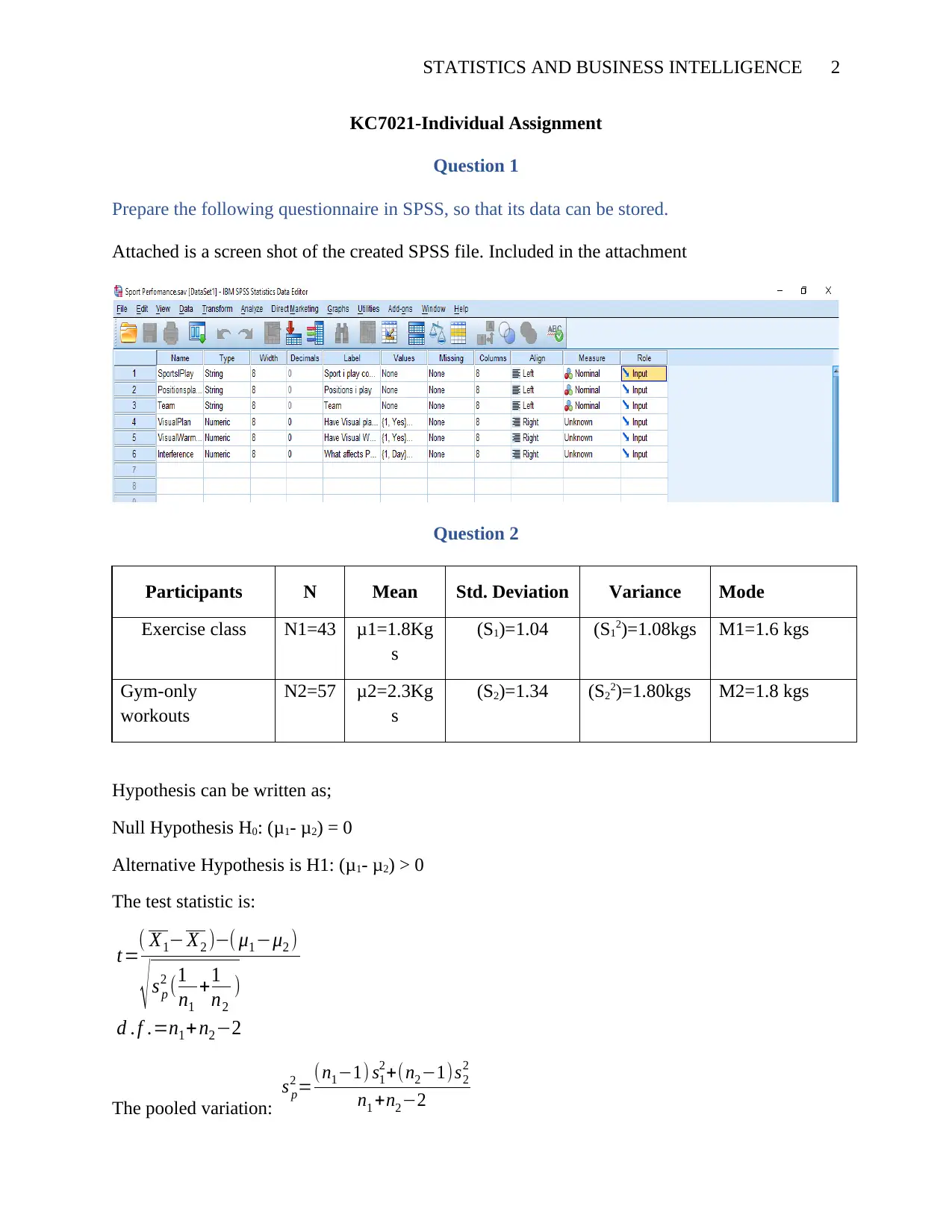
Prepare the following questionnaire in SPSS, so that its data can be stored.
Attached is a screen shot of the created SPSS file. Included in the attachment
Question 2
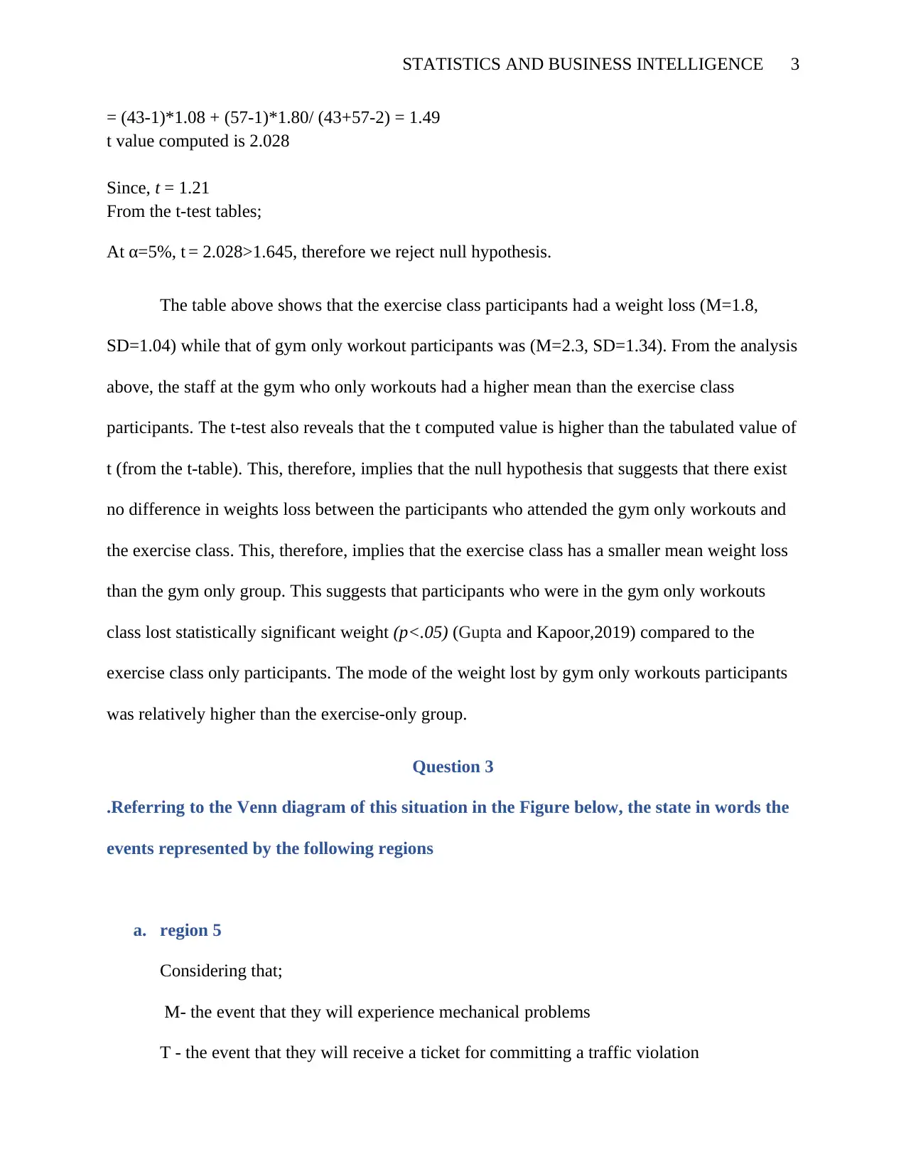
Participants N Mean Std. Deviation Variance Mode
Exercise class N1=43 μ1=1.8Kg
s
(S1)=1.04 (S12)=1.08kgs M1=1.6 kgs
Gym-only
workouts
N2=57 μ2=2.3Kg
s
(S2)=1.34 (S22)=1.80kgs M2=1.8 kgs
Hypothesis can be written as;
Null Hypothesis H0: (μ1- μ2) = 0
Alternative Hypothesis is H1: (μ1- μ2) > 0
The test statistic is:
t=( X1− X2 )−( μ1−μ2 )
√ s p
2 (1
n1
+1
n2
)
d . f .=n1+ n2−2
The pooled variation:
s p
2 =(n1−1) s1
2+(n2−1)s2
2
n1 +n2−2
KC7021-Individual Assignment
Question 1
Prepare the following questionnaire in SPSS, so that its data can be stored.
Attached is a screen shot of the created SPSS file. Included in the attachment
Question 2
Participants N Mean Std. Deviation Variance Mode
Exercise class N1=43 μ1=1.8Kg
s
(S1)=1.04 (S12)=1.08kgs M1=1.6 kgs
Gym-only
workouts
N2=57 μ2=2.3Kg
s
(S2)=1.34 (S22)=1.80kgs M2=1.8 kgs
Hypothesis can be written as;
Null Hypothesis H0: (μ1- μ2) = 0
Alternative Hypothesis is H1: (μ1- μ2) > 0
The test statistic is:
t=( X1− X2 )−( μ1−μ2 )
√ s p
2 (1
n1
+1
n2
)
d . f .=n1+ n2−2
The pooled variation:
s p
2 =(n1−1) s1
2+(n2−1)s2
2
n1 +n2−2
STATISTICS AND BUSINESS INTELLIGENCE 3
= (43-1)*1.08 + (57-1)*1.80/ (43+57-2) = 1.49
t value computed is 2.028
Since, t = 1.21
From the t-test tables;
At α=5%, t = 2.028>1.645, therefore we reject null hypothesis.
The table above shows that the exercise class participants had a weight loss (M=1.8,
SD=1.04) while that of gym only workout participants was (M=2.3, SD=1.34). From the analysis
above, the staff at the gym who only workouts had a higher mean than the exercise class
participants. The t-test also reveals that the t computed value is higher than the tabulated value of
t (from the t-table). This, therefore, implies that the null hypothesis that suggests that there exist
no difference in weights loss between the participants who attended the gym only workouts and
the exercise class. This, therefore, implies that the exercise class has a smaller mean weight loss
than the gym only group. This suggests that participants who were in the gym only workouts
class lost statistically significant weight (p<.05) (Gupta and Kapoor,2019) compared to the
exercise class only participants. The mode of the weight lost by gym only workouts participants
was relatively higher than the exercise-only group.
Question 3
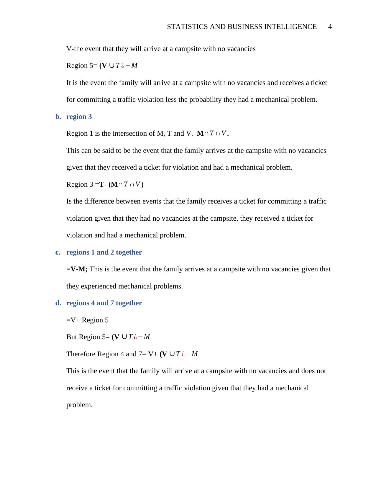
.Referring to the Venn diagram of this situation in the Figure below, the state in words the
events represented by the following regions
a. region 5
Considering that;
M- the event that they will experience mechanical problems
T - the event that they will receive a ticket for committing a traffic violation
= (43-1)*1.08 + (57-1)*1.80/ (43+57-2) = 1.49
t value computed is 2.028
Since, t = 1.21
From the t-test tables;
At α=5%, t = 2.028>1.645, therefore we reject null hypothesis.
The table above shows that the exercise class participants had a weight loss (M=1.8,
SD=1.04) while that of gym only workout participants was (M=2.3, SD=1.34). From the analysis
above, the staff at the gym who only workouts had a higher mean than the exercise class
participants. The t-test also reveals that the t computed value is higher than the tabulated value of
t (from the t-table). This, therefore, implies that the null hypothesis that suggests that there exist
no difference in weights loss between the participants who attended the gym only workouts and
the exercise class. This, therefore, implies that the exercise class has a smaller mean weight loss
than the gym only group. This suggests that participants who were in the gym only workouts
class lost statistically significant weight (p<.05) (Gupta and Kapoor,2019) compared to the
exercise class only participants. The mode of the weight lost by gym only workouts participants
was relatively higher than the exercise-only group.
Question 3
.Referring to the Venn diagram of this situation in the Figure below, the state in words the
events represented by the following regions
a. region 5
Considering that;
M- the event that they will experience mechanical problems
T - the event that they will receive a ticket for committing a traffic violation
⊘ This is a preview!⊘
Do you want full access?
Subscribe today to unlock all pages.
Trusted by 1+ million students worldwide
STATISTICS AND BUSINESS INTELLIGENCE 4
V-the event that they will arrive at a campsite with no vacancies
Region 5= (V ∪ T ¿−M
It is the event the family will arrive at a campsite with no vacancies and receives a ticket
for committing a traffic violation less the probability they had a mechanical problem.
b. region 3
Region 1 is the intersection of M, T and V. M∩T ∩V .
This can be said to be the event that the family arrives at the campsite with no vacancies
given that they received a ticket for violation and had a mechanical problem.
Region 3 =T- (M∩T ∩V )
Is the difference between events that the family receives a ticket for committing a traffic
violation given that they had no vacancies at the campsite, they received a ticket for
violation and had a mechanical problem.
c. regions 1 and 2 together
=V-M; This is the event that the family arrives at a campsite with no vacancies given that
they experienced mechanical problems.
d. regions 4 and 7 together
=V+ Region 5
But Region 5= (V ∪ T ¿−M
Therefore Region 4 and 7= V+ (V ∪T ¿−M
This is the event that the family will arrive at a campsite with no vacancies and does not
receive a ticket for committing a traffic violation given that they had a mechanical
problem.
Paraphrase This Document
Need a fresh take? Get an instant paraphrase of this document with our AI Paraphraser
STATISTICS AND BUSINESS INTELLIGENCE 5
e. regions 3, 6, 7, and 8 together
= Universal set+ region 6+ region 3+ region7
The remaining from this is the subset M.This is the event that the family will experience
mechanical problems
Question 4
a. What is the probability that an LCD TV is in a bedroom?
It is the probability that LCD TV is in the adult bedroom and child bedroom and other
bedroom
Probability= (B1*B2+B3)
P(LCD IN BEDROOM) = 0.13*0.08*0.11=0.001144
b. What is the probability that it is not in a bedroom?
=1- P (LCD IN BEDROOM)= 1-0.001144=0.9989
c. Suppose a household is selected at random from households with an LCD TV; in
what room would you expect to find an LCD TV
The probability that the LCD TV is in the Adult bedroom: 0.13, Child bedroom: 0.08,
Other bedroom: 0.11, Office or den: 0.40 other rooms: 0.28.
Since it is randomly selected, office or den tend to have the highest probability of having
been selected. Out of the 4 option available, it is true to say the each option has a
probability of ¼ multiplied by its actual probability i.e. ¼*0.4=0.1
Question 5
The probability that an iPhone will survive a shock test is 3/4. Find the probability that
exactly 2 of the next 4 iPhones tested survive. These tests are independent
STATISTICS AND BUSINESS INTELLIGENCE 6
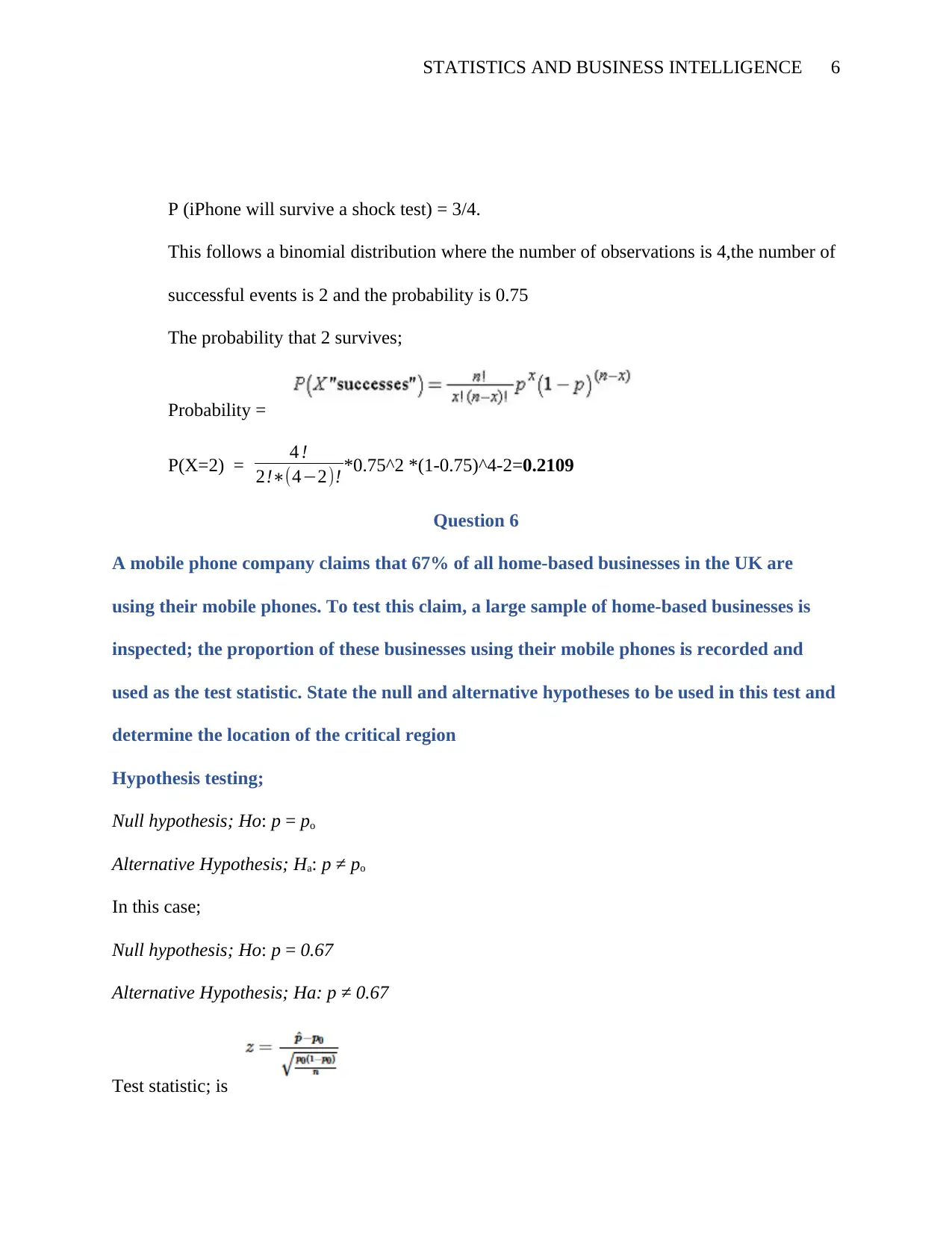
P (iPhone will survive a shock test) = 3/4.
This follows a binomial distribution where the number of observations is 4,the number of
successful events is 2 and the probability is 0.75
The probability that 2 survives;
Probability =
P(X=2) = 4 !
2!∗(4−2)! *0.75^2 *(1-0.75)^4-2=0.2109
Question 6
A mobile phone company claims that 67% of all home-based businesses in the UK are
using their mobile phones. To test this claim, a large sample of home-based businesses is
inspected; the proportion of these businesses using their mobile phones is recorded and
used as the test statistic. State the null and alternative hypotheses to be used in this test and
determine the location of the critical region
Hypothesis testing;
Null hypothesis; Ho: p = po
Alternative Hypothesis; Ha: p ≠ po
In this case;
Null hypothesis; Ho: p = 0.67
Alternative Hypothesis; Ha: p ≠ 0.67
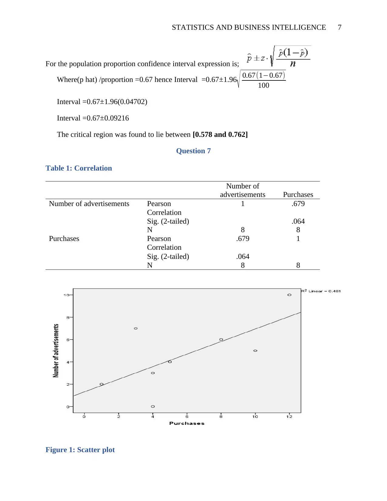
Test statistic; is
P (iPhone will survive a shock test) = 3/4.
This follows a binomial distribution where the number of observations is 4,the number of
successful events is 2 and the probability is 0.75
The probability that 2 survives;
Probability =
P(X=2) = 4 !
2!∗(4−2)! *0.75^2 *(1-0.75)^4-2=0.2109
Question 6
A mobile phone company claims that 67% of all home-based businesses in the UK are
using their mobile phones. To test this claim, a large sample of home-based businesses is
inspected; the proportion of these businesses using their mobile phones is recorded and
used as the test statistic. State the null and alternative hypotheses to be used in this test and
determine the location of the critical region
Hypothesis testing;
Null hypothesis; Ho: p = po
Alternative Hypothesis; Ha: p ≠ po
In this case;
Null hypothesis; Ho: p = 0.67
Alternative Hypothesis; Ha: p ≠ 0.67
Test statistic; is
⊘ This is a preview!⊘
Do you want full access?
Subscribe today to unlock all pages.
Trusted by 1+ million students worldwide
STATISTICS AND BUSINESS INTELLIGENCE 7
For the population proportion confidence interval expression is;
Where(p hat) /proportion =0.67 hence Interval =0.67±1.96
√ 0.67(1−0.67)
100
Interval =0.67±1.96(0.04702)
Interval =0.67±0.09216
The critical region was found to lie between [0.578 and 0.762]
Question 7
Table 1: Correlation
Number of
advertisements Purchases
Number of advertisements Pearson
Correlation
1 .679
Sig. (2-tailed) .064
N 8 8
Purchases Pearson
Correlation
.679 1
Sig. (2-tailed) .064
N 8 8
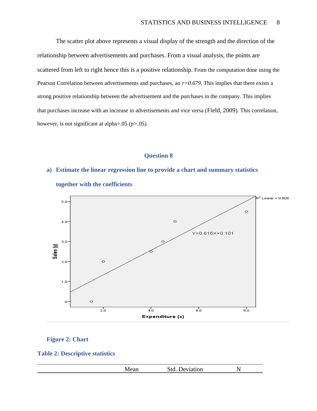
Figure 1: Scatter plot
For the population proportion confidence interval expression is;
Where(p hat) /proportion =0.67 hence Interval =0.67±1.96
√ 0.67(1−0.67)
100
Interval =0.67±1.96(0.04702)
Interval =0.67±0.09216
The critical region was found to lie between [0.578 and 0.762]
Question 7
Table 1: Correlation
Number of
advertisements Purchases
Number of advertisements Pearson
Correlation
1 .679
Sig. (2-tailed) .064
N 8 8
Purchases Pearson
Correlation
.679 1
Sig. (2-tailed) .064
N 8 8
Figure 1: Scatter plot
Paraphrase This Document
Need a fresh take? Get an instant paraphrase of this document with our AI Paraphraser
STATISTICS AND BUSINESS INTELLIGENCE 8
The scatter plot above represents a visual display of the strength and the direction of the
relationship between advertisements and purchases. From a visual analysis, the points are
scattered from left to right hence this is a positive relationship. From the computation done using the
Pearson Correlation between advertisements and purchases, an r=0.679. This implies that there exists a
strong positive relationship between the advertisement and the purchases in the company. This implies
that purchases increase with an increase in advertisements and vice versa (Field, 2009). This correlation,
however, is not significant at alpha=.05 (p>.05).
Question 8
a) Estimate the linear regression line to provide a chart and summary statistics
together with the coefficients
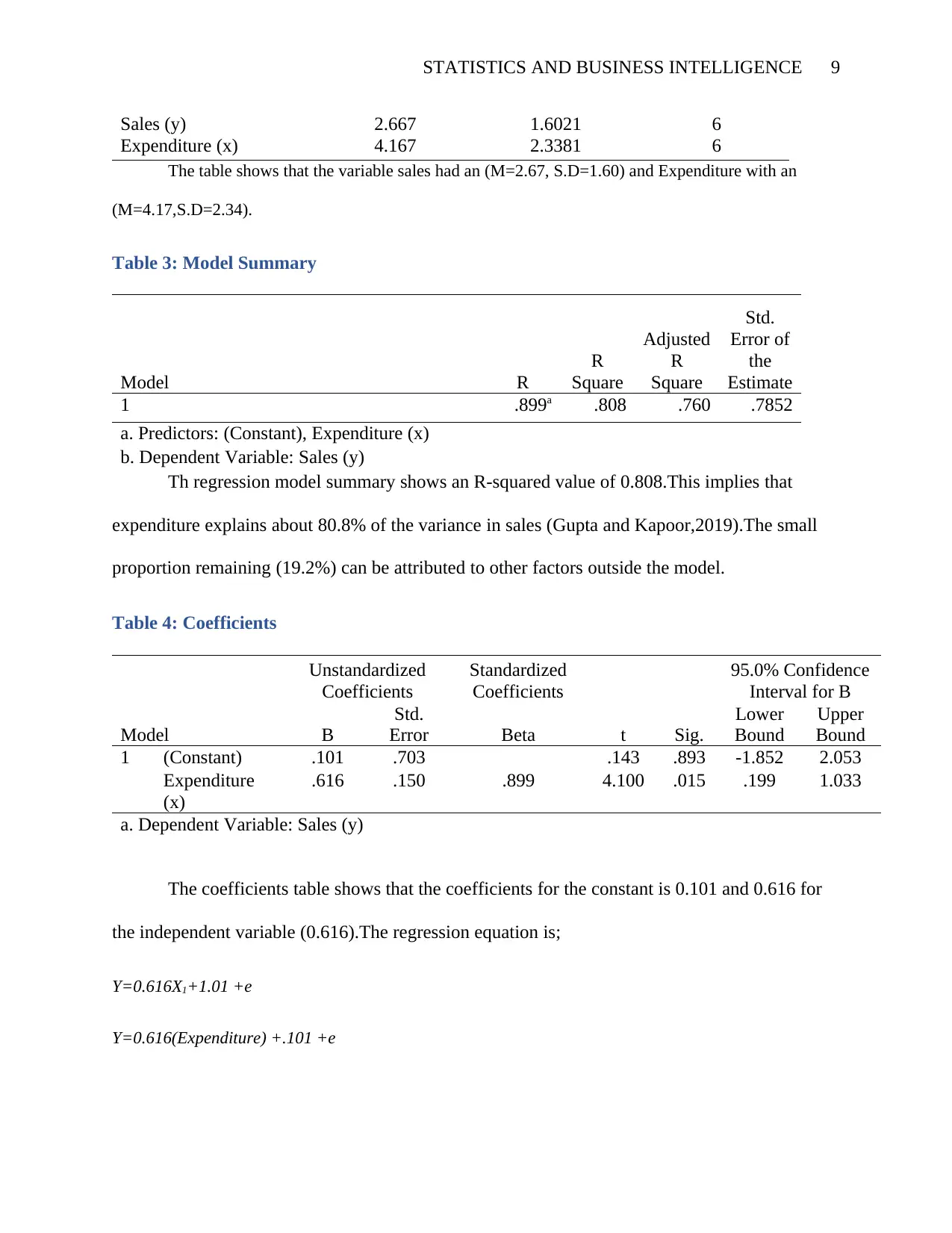
Figure 2: Chart
Table 2: Descriptive statistics
Mean Std. Deviation N
The scatter plot above represents a visual display of the strength and the direction of the
relationship between advertisements and purchases. From a visual analysis, the points are
scattered from left to right hence this is a positive relationship. From the computation done using the
Pearson Correlation between advertisements and purchases, an r=0.679. This implies that there exists a
strong positive relationship between the advertisement and the purchases in the company. This implies
that purchases increase with an increase in advertisements and vice versa (Field, 2009). This correlation,
however, is not significant at alpha=.05 (p>.05).
Question 8
a) Estimate the linear regression line to provide a chart and summary statistics
together with the coefficients
Figure 2: Chart
Table 2: Descriptive statistics
Mean Std. Deviation N
STATISTICS AND BUSINESS INTELLIGENCE 9
Sales (y) 2.667 1.6021 6
Expenditure (x) 4.167 2.3381 6
The table shows that the variable sales had an (M=2.67, S.D=1.60) and Expenditure with an
(M=4.17,S.D=2.34).
Table 3: Model Summary
Model R
R
Square
Adjusted
R
Square
Std.
Error of
the
Estimate
1 .899a .808 .760 .7852
a. Predictors: (Constant), Expenditure (x)
b. Dependent Variable: Sales (y)
Th regression model summary shows an R-squared value of 0.808.This implies that
expenditure explains about 80.8% of the variance in sales (Gupta and Kapoor,2019).The small
proportion remaining (19.2%) can be attributed to other factors outside the model.
Table 4: Coefficients
Model
Unstandardized
Coefficients
Standardized
Coefficients
t Sig.
95.0% Confidence
Interval for B
B
Std.
Error Beta
Lower
Bound
Upper
Bound
1 (Constant) .101 .703 .143 .893 -1.852 2.053
Expenditure
(x)
.616 .150 .899 4.100 .015 .199 1.033
a. Dependent Variable: Sales (y)
The coefficients table shows that the coefficients for the constant is 0.101 and 0.616 for
the independent variable (0.616).The regression equation is;
Y=0.616X1+1.01 +e
Y=0.616(Expenditure) +.101 +e
⊘ This is a preview!⊘
Do you want full access?
Subscribe today to unlock all pages.
Trusted by 1+ million students worldwide
STATISTICS AND BUSINESS INTELLIGENCE 10
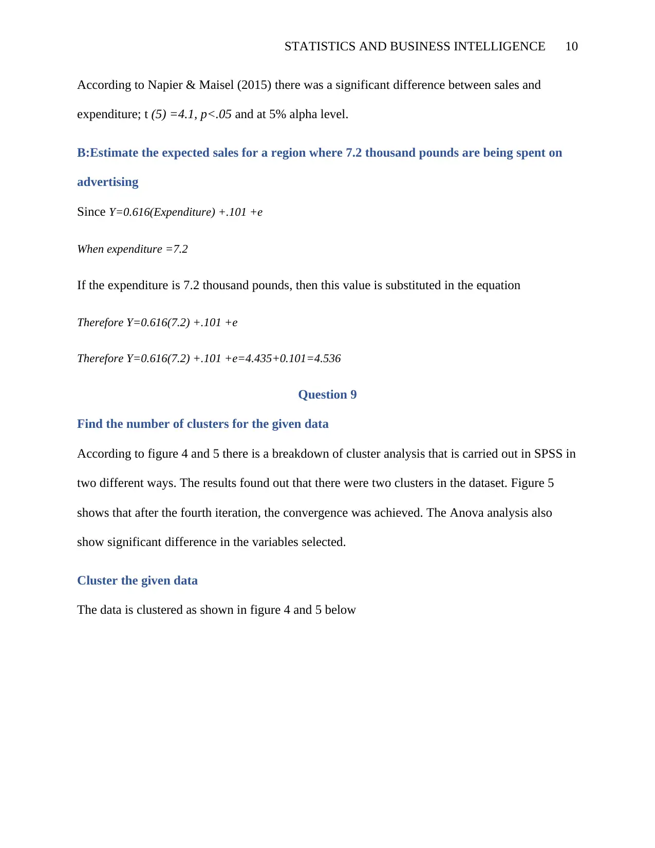
According to Napier & Maisel (2015) there was a significant difference between sales and
expenditure; t (5) =4.1, p<.05 and at 5% alpha level.
B:Estimate the expected sales for a region where 7.2 thousand pounds are being spent on
advertising
Since Y=0.616(Expenditure) +.101 +e
When expenditure =7.2
If the expenditure is 7.2 thousand pounds, then this value is substituted in the equation
Therefore Y=0.616(7.2) +.101 +e
Therefore Y=0.616(7.2) +.101 +e=4.435+0.101=4.536
Question 9
Find the number of clusters for the given data
According to figure 4 and 5 there is a breakdown of cluster analysis that is carried out in SPSS in
two different ways. The results found out that there were two clusters in the dataset. Figure 5
shows that after the fourth iteration, the convergence was achieved. The Anova analysis also
show significant difference in the variables selected.
Cluster the given data
The data is clustered as shown in figure 4 and 5 below
Paraphrase This Document
Need a fresh take? Get an instant paraphrase of this document with our AI Paraphraser
STATISTICS AND BUSINESS INTELLIGENCE 11
Question 10
You are a director of a major manufacturing organisation, and collecting various pieces of
information for your potential customers, such as on one of your major customers who is
based in London, will require delivery lorries to travel the length of the M1. You will
investigate the speed on this road using the data available at
http://www.trafficengland.com/traffic-report
You should only use the source specified. You will need to adopt a sampling approach and
credit will be given for schemes which show you have considered how to apply the
principles of sampling to obtain the best results with the smallest possible dataset.
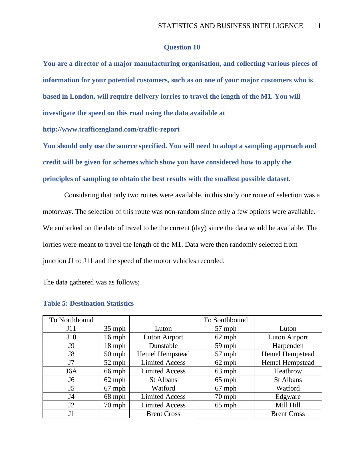
Considering that only two routes were available, in this study our route of selection was a
motorway. The selection of this route was non-random since only a few options were available.
We embarked on the date of travel to be the current (day) since the data would be available. The
lorries were meant to travel the length of the M1. Data were then randomly selected from
junction J1 to J11 and the speed of the motor vehicles recorded.
The data gathered was as follows;
Table 5: Destination Statistics
To Northbound To Southbound
J11 35 mph Luton 57 mph Luton
J10 16 mph Luton Airport 62 mph Luton Airport
J9 18 mph Dunstable 59 mph Harpenden
J8 50 mph Hemel Hempstead 57 mph Hemel Hempstead
J7 52 mph Limited Access 62 mph Hemel Hempstead
J6A 66 mph Limited Access 63 mph Heathrow
J6 62 mph St Albans 65 mph St Albans
J5 67 mph Watford 67 mph Watford
J4 68 mph Limited Access 70 mph Edgware
J2 70 mph Limited Access 65 mph Mill Hill
J1 Brent Cross Brent Cross
Question 10
You are a director of a major manufacturing organisation, and collecting various pieces of
information for your potential customers, such as on one of your major customers who is
based in London, will require delivery lorries to travel the length of the M1. You will
investigate the speed on this road using the data available at
http://www.trafficengland.com/traffic-report
You should only use the source specified. You will need to adopt a sampling approach and
credit will be given for schemes which show you have considered how to apply the
principles of sampling to obtain the best results with the smallest possible dataset.
Considering that only two routes were available, in this study our route of selection was a
motorway. The selection of this route was non-random since only a few options were available.
We embarked on the date of travel to be the current (day) since the data would be available. The
lorries were meant to travel the length of the M1. Data were then randomly selected from
junction J1 to J11 and the speed of the motor vehicles recorded.
The data gathered was as follows;
Table 5: Destination Statistics
To Northbound To Southbound
J11 35 mph Luton 57 mph Luton
J10 16 mph Luton Airport 62 mph Luton Airport
J9 18 mph Dunstable 59 mph Harpenden
J8 50 mph Hemel Hempstead 57 mph Hemel Hempstead
J7 52 mph Limited Access 62 mph Hemel Hempstead
J6A 66 mph Limited Access 63 mph Heathrow
J6 62 mph St Albans 65 mph St Albans
J5 67 mph Watford 67 mph Watford
J4 68 mph Limited Access 70 mph Edgware
J2 70 mph Limited Access 65 mph Mill Hill
J1 Brent Cross Brent Cross
STATISTICS AND BUSINESS INTELLIGENCE 12
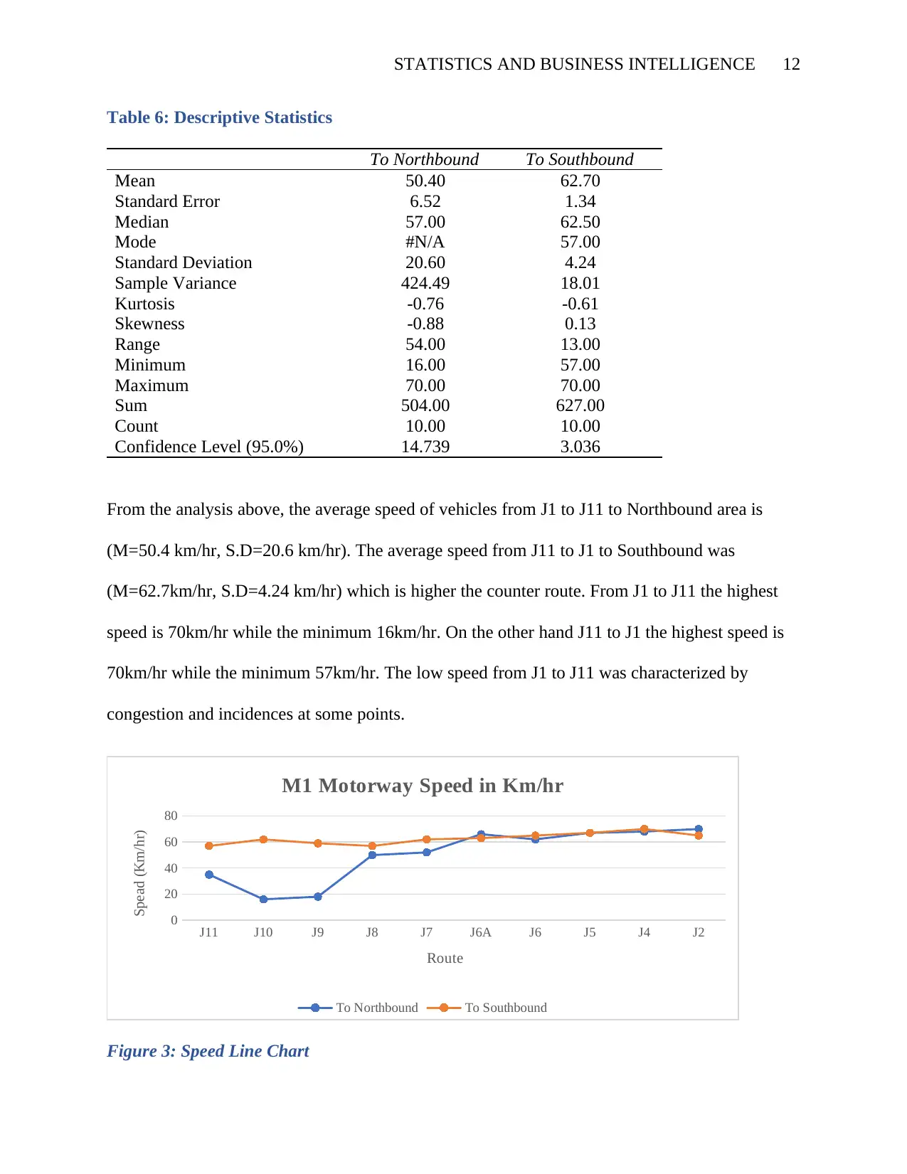
Table 6: Descriptive Statistics
To Northbound To Southbound
Mean 50.40 62.70
Standard Error 6.52 1.34
Median 57.00 62.50
Mode #N/A 57.00
Standard Deviation 20.60 4.24
Sample Variance 424.49 18.01
Kurtosis -0.76 -0.61
Skewness -0.88 0.13
Range 54.00 13.00
Minimum 16.00 57.00
Maximum 70.00 70.00
Sum 504.00 627.00
Count 10.00 10.00
Confidence Level (95.0%) 14.739 3.036
From the analysis above, the average speed of vehicles from J1 to J11 to Northbound area is
(M=50.4 km/hr, S.D=20.6 km/hr). The average speed from J11 to J1 to Southbound was
(M=62.7km/hr, S.D=4.24 km/hr) which is higher the counter route. From J1 to J11 the highest
speed is 70km/hr while the minimum 16km/hr. On the other hand J11 to J1 the highest speed is
70km/hr while the minimum 57km/hr. The low speed from J1 to J11 was characterized by
congestion and incidences at some points.
J11 J10 J9 J8 J7 J6A J6 J5 J4 J2
0
20
40
60
80
M1 Motorway Speed in Km/hr
To Northbound To Southbound
Route
Spead (Km/hr)
Figure 3: Speed Line Chart
⊘ This is a preview!⊘
Do you want full access?
Subscribe today to unlock all pages.
Trusted by 1+ million students worldwide
1 out of 16
Your All-in-One AI-Powered Toolkit for Academic Success.
+13062052269
info@desklib.com
Available 24*7 on WhatsApp / Email
![[object Object]](/_next/static/media/star-bottom.7253800d.svg)
Unlock your academic potential
Copyright © 2020–2026 A2Z Services. All Rights Reserved. Developed and managed by ZUCOL.