BUGEN1502: Business Statistics Assignment 2 - Semester 2, 2019

This assignment solution addresses a statistics problem related to the average arrival time of packages in Australia, based on data from Hong Kong. The solution begins with a histogram analysis, revealing the distribution's characteristics, and calculates descriptive statistics to understand central tendency and variability. It then proceeds to construct confidence intervals for population means, both with known and unknown standard deviations. The assignment further delves into hypothesis testing, outlining the procedures, test statistics, and decision rules to determine if the mean arrival time has changed or exceeds a certain value. The solution also explains the significance of p-values in hypothesis testing, comparing them to critical value approaches and clarifying their implications on rejecting null hypotheses. The assignment concludes with a discussion on the relationship between p-values and statistical significance.

Running head: STATISTICS
Statistics
Name of the Student
Name of the University
Course ID

1STATISTICS
Table of Contents
Question 1........................................................................................................................................2
Question 2........................................................................................................................................4
Question 3........................................................................................................................................5
Question 4........................................................................................................................................7
References........................................................................................................................................9

2STATISTICS
Question 1
1)
0-3 3-6 6-9 9-12 12-15 15-18 18-21 21-24 24-27 27-30 30-33
0
10
20
30
40
50
60
Histogram
Class
Frequency
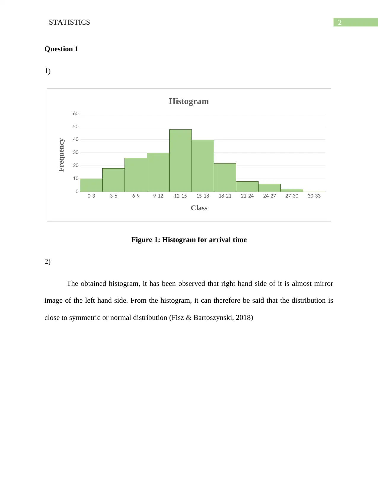
Figure 1: Histogram for arrival time
2)
The obtained histogram, it has been observed that right hand side of it is almost mirror
image of the left hand side. From the histogram, it can therefore be said that the distribution is
close to symmetric or normal distribution (Fisz & Bartoszynski, 2018)

3STATISTICS
3)
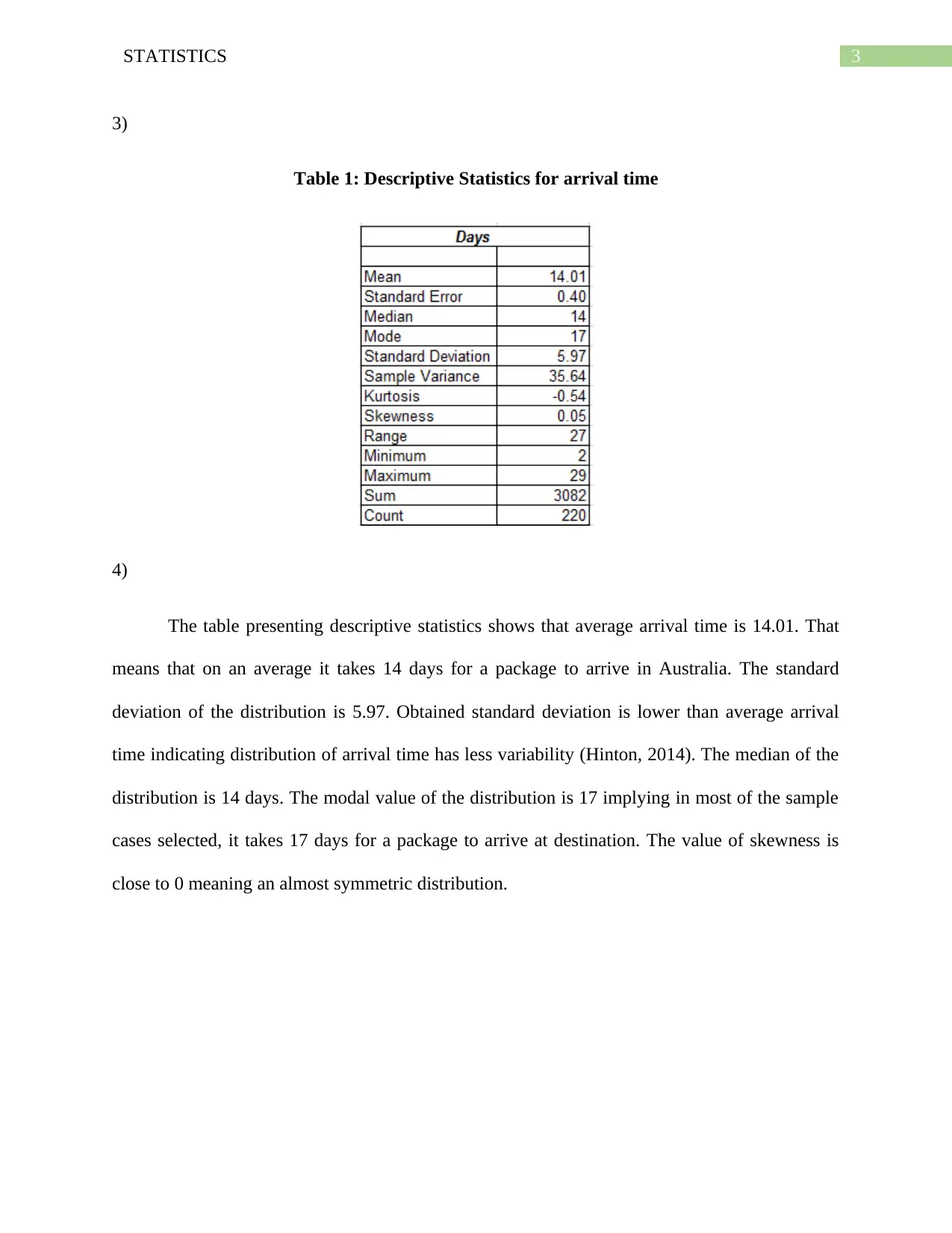
Table 1: Descriptive Statistics for arrival time
4)
The table presenting descriptive statistics shows that average arrival time is 14.01. That
means that on an average it takes 14 days for a package to arrive in Australia. The standard
deviation of the distribution is 5.97. Obtained standard deviation is lower than average arrival
time indicating distribution of arrival time has less variability (Hinton, 2014). The median of the
distribution is 14 days. The modal value of the distribution is 17 implying in most of the sample
cases selected, it takes 17 days for a package to arrive at destination. The value of skewness is
close to 0 meaning an almost symmetric distribution.

4STATISTICS
Question 2
1)
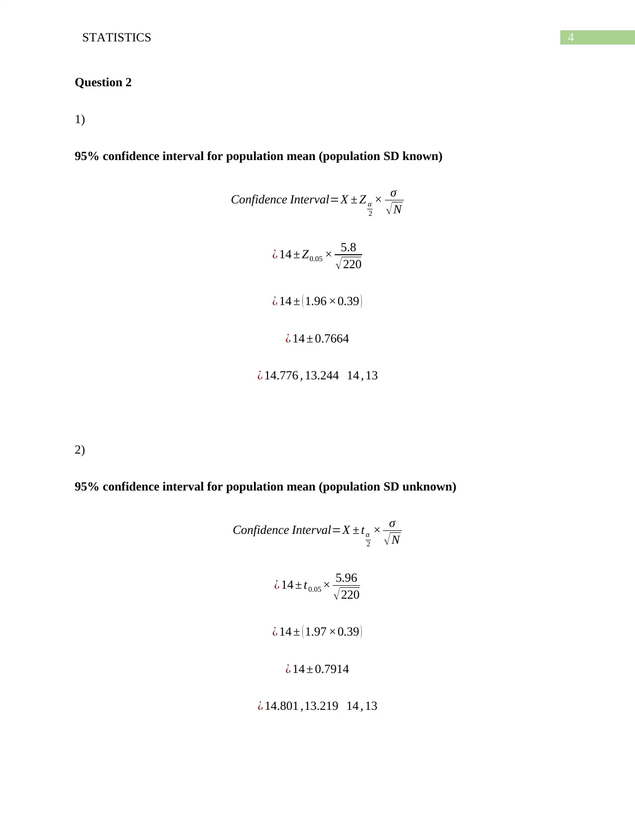
95% confidence interval for population mean (population SD known)
Confidence Interval=X ± Z α
2
× σ
√N
¿ 14 ± Z0.05 × 5.8
√ 220
¿ 14 ± ( 1.96 ×0.39 )
¿ 14 ± 0.7664
¿ 14.776 , 13.244 14 , 13
2)
95% confidence interval for population mean (population SD unknown)
Confidence Interval=X ± tα
2
× σ
√N
¿ 14 ± t0.05 × 5.96
√220
¿ 14 ± ( 1.97 ×0.39 )
¿ 14 ± 0.7914
¿ 14.801 ,13.219 14 , 13

5STATISTICS

6STATISTICS
Question 3
1)
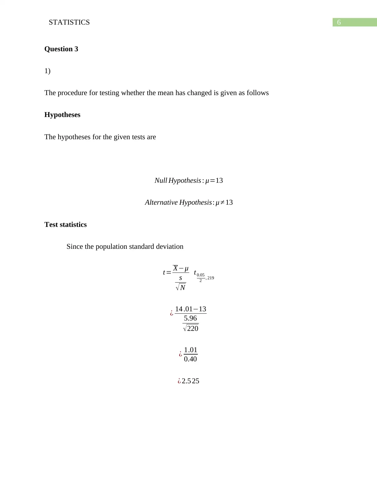
The procedure for testing whether the mean has changed is given as follows
Hypotheses
The hypotheses for the given tests are
Null Hypothesis : μ=13
Alternative Hypothesis: μ ≠ 13
Test statistics
Since the population standard deviation
t= X−μ
s
√ N
t0.05
2 , 219
¿ 14 .01−13
5.96
√ 220
¿ 1.01
0.40
¿ 2.5 25

7STATISTICS
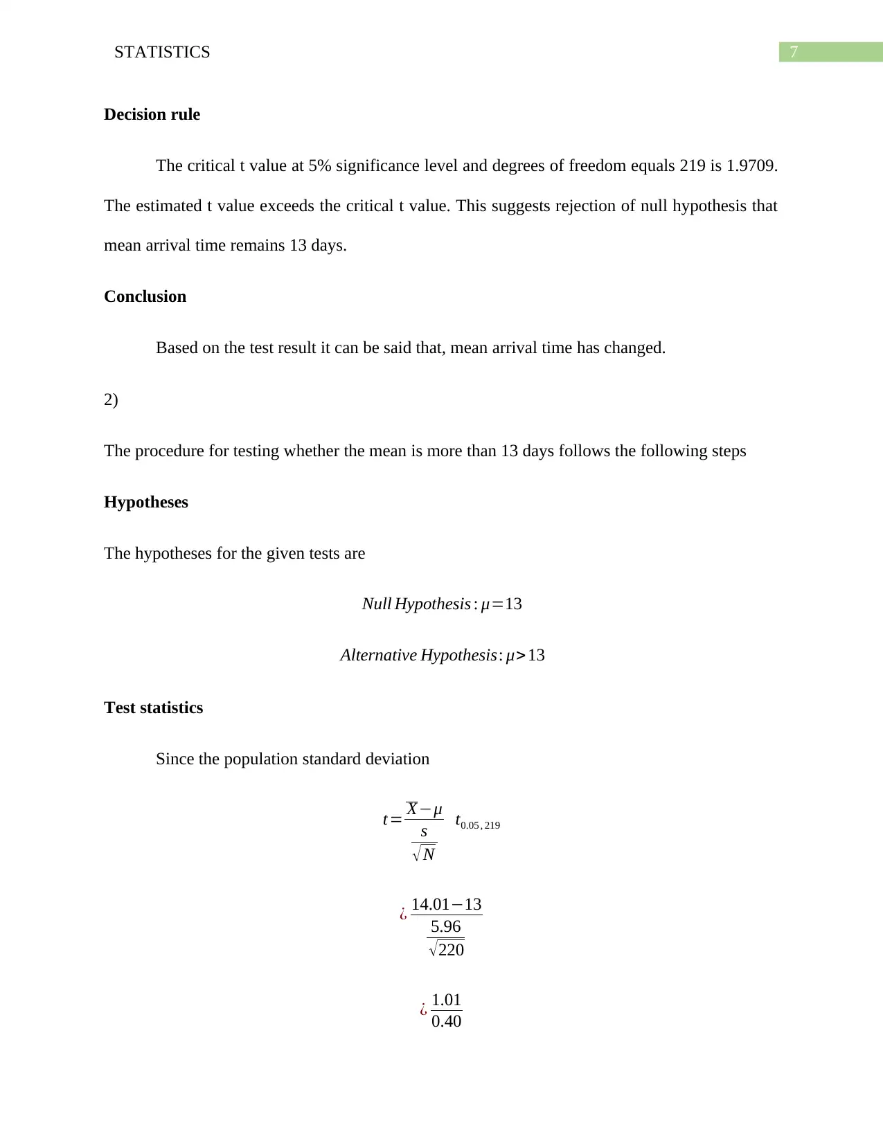
Decision rule
The critical t value at 5% significance level and degrees of freedom equals 219 is 1.9709.
The estimated t value exceeds the critical t value. This suggests rejection of null hypothesis that
mean arrival time remains 13 days.
Conclusion
Based on the test result it can be said that, mean arrival time has changed.
2)
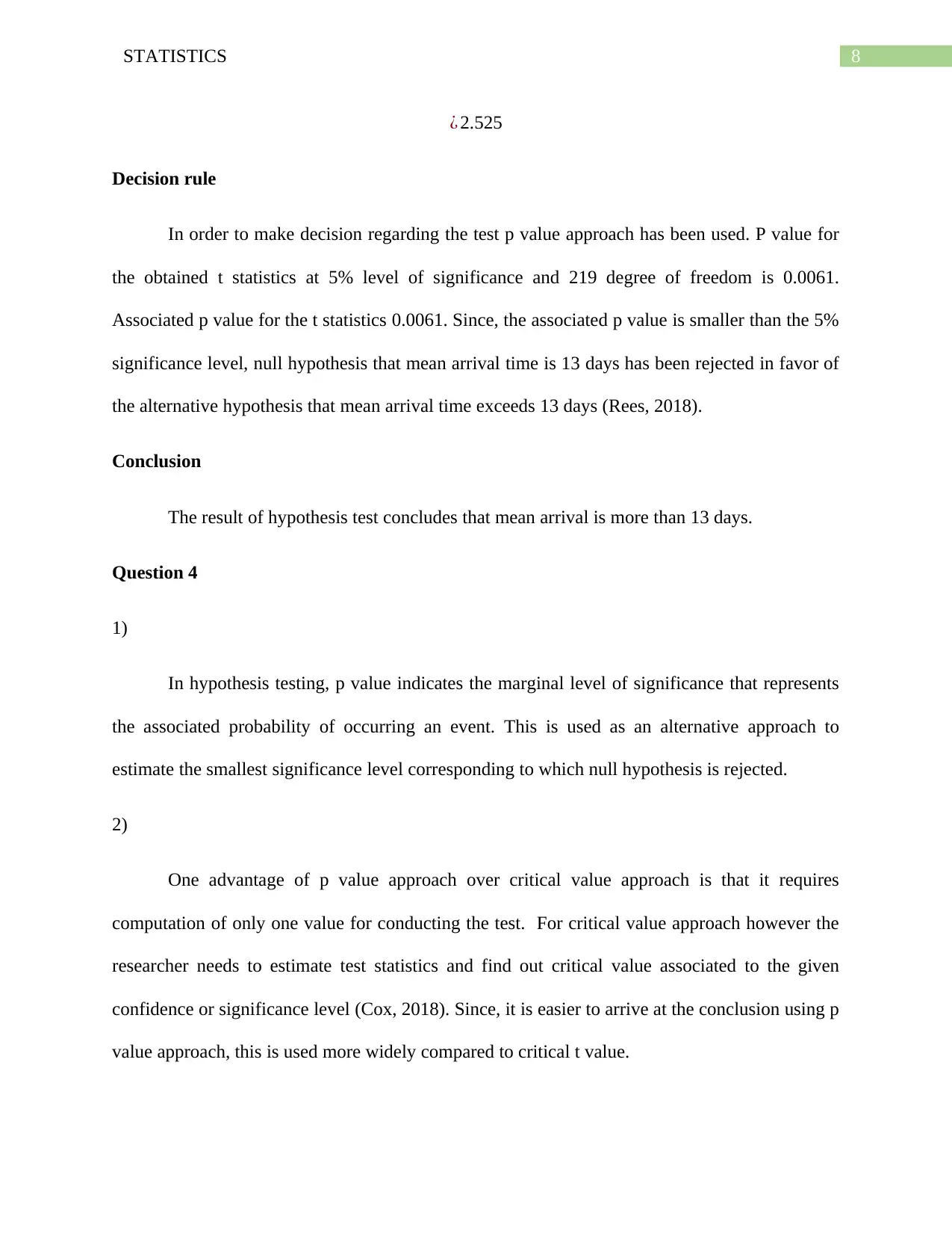
The procedure for testing whether the mean is more than 13 days follows the following steps
Hypotheses
The hypotheses for the given tests are
Null Hypothesis : μ=13
Alternative Hypothesis: μ>13
Test statistics
Since the population standard deviation
t= X−μ
s
√ N
t0.05 , 219
¿ 14.01−13
5.96
√220
¿ 1.01
0.40

8STATISTICS
¿ 2.525
Decision rule
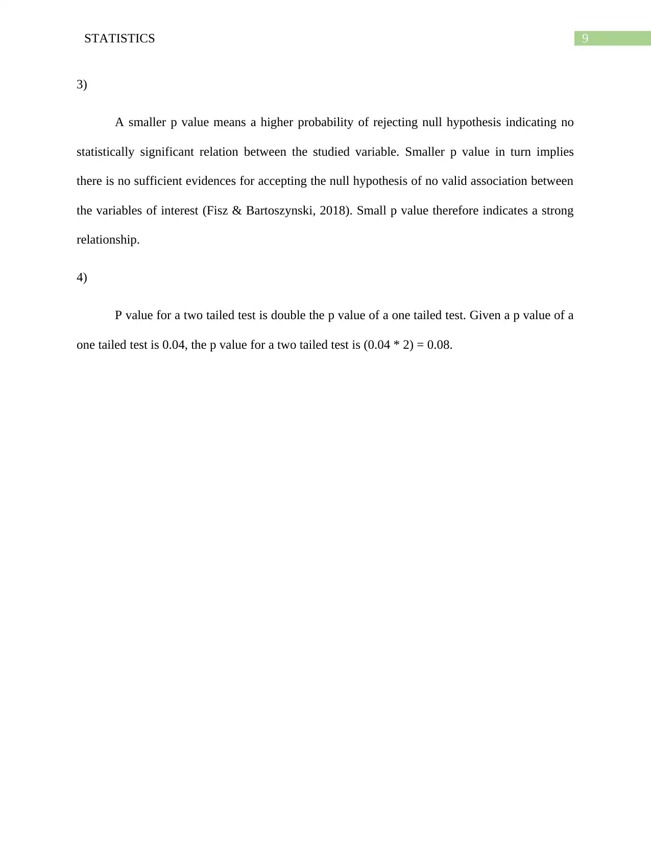
In order to make decision regarding the test p value approach has been used. P value for
the obtained t statistics at 5% level of significance and 219 degree of freedom is 0.0061.
Associated p value for the t statistics 0.0061. Since, the associated p value is smaller than the 5%
significance level, null hypothesis that mean arrival time is 13 days has been rejected in favor of
the alternative hypothesis that mean arrival time exceeds 13 days (Rees, 2018).
Conclusion
The result of hypothesis test concludes that mean arrival is more than 13 days.
Question 4
1)
In hypothesis testing, p value indicates the marginal level of significance that represents
the associated probability of occurring an event. This is used as an alternative approach to
estimate the smallest significance level corresponding to which null hypothesis is rejected.
2)
One advantage of p value approach over critical value approach is that it requires
computation of only one value for conducting the test. For critical value approach however the
researcher needs to estimate test statistics and find out critical value associated to the given
confidence or significance level (Cox, 2018). Since, it is easier to arrive at the conclusion using p
value approach, this is used more widely compared to critical t value.

9STATISTICS
3)
A smaller p value means a higher probability of rejecting null hypothesis indicating no
statistically significant relation between the studied variable. Smaller p value in turn implies
there is no sufficient evidences for accepting the null hypothesis of no valid association between
the variables of interest (Fisz & Bartoszynski, 2018). Small p value therefore indicates a strong
relationship.
4)
P value for a two tailed test is double the p value of a one tailed test. Given a p value of a
one tailed test is 0.04, the p value for a two tailed test is (0.04 * 2) = 0.08.

10STATISTICS
References
Cox, D. R. (2018). Applied statistics-principles and examples. Routledge.
Fisz, M., & Bartoszynski, R. (2018). Probability theory and mathematical statistics (Vol. 3). J.
wiley.
Hinton, P. R. (2014). Statistics explained. Routledge.
Rees, D. G. (2018). Essential statistics. Chapman and Hall/CRC.