Statistics Homework: Analysis of Variance, Regression and Data

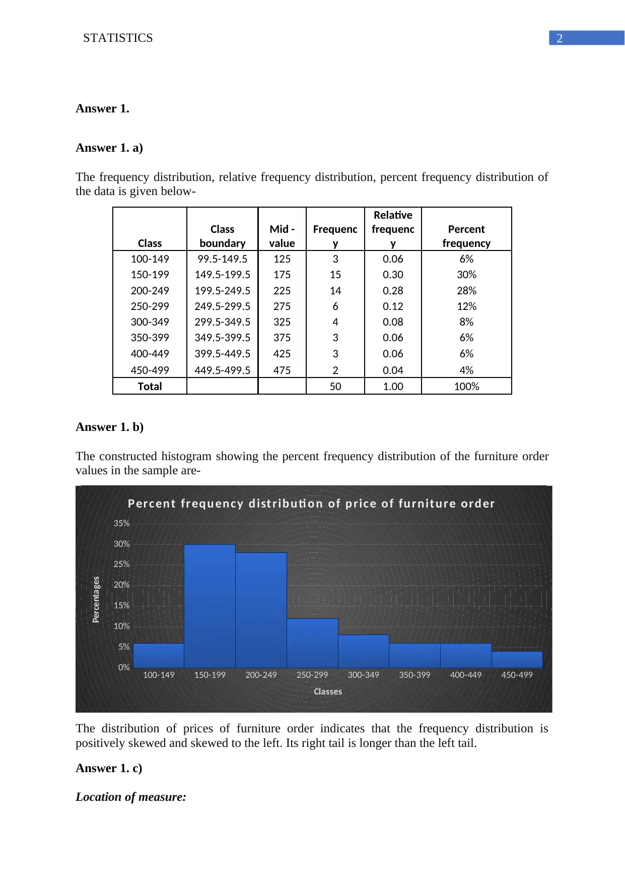
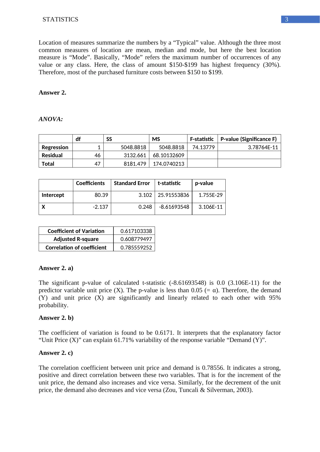
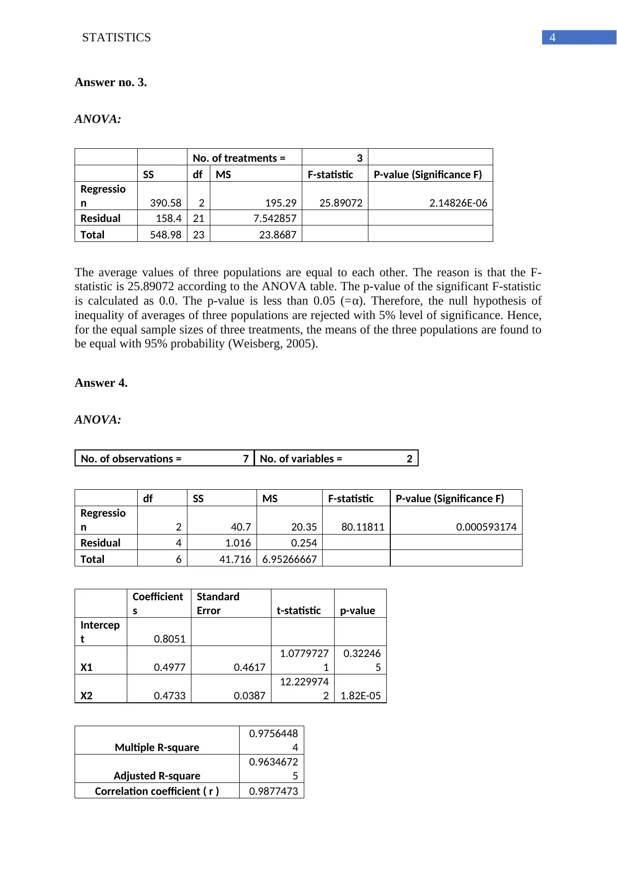
This statistics assignment presents a comprehensive analysis of various statistical concepts. It begins with a frequency distribution analysis, including calculations of relative and percent frequencies, and the construction of a histogram to visualize the data. The assignment then delves into regression analysis, providing ANOVA tables, coefficient of variation, and correlation coefficients to assess the relationship between variables. The analysis includes interpretations of p-values and t-statistics to determine statistical significance. Furthermore, the assignment explores ANOVA to compare the means of multiple populations, determining whether the means are equal. Finally, the assignment culminates in a multiple regression analysis, estimating a linear regression equation and interpreting the coefficients to understand the impact of independent variables on the dependent variable. The assignment covers concepts of statistical significance, correlation, and interpretation of regression models.

Running head: STATISTICS
Statistics
Name of the Student
Name of the University
Author’s Note

1STATISTICS
Table of Contents
Answer 1....................................................................................................................................2
Answer 1. a)...........................................................................................................................2
Answer 1. b)...........................................................................................................................2
Answer 1. c)...........................................................................................................................2
Answer 2....................................................................................................................................3
Answer 2. a)...........................................................................................................................3
Answer 2. b)...........................................................................................................................3
Answer 2. c)...........................................................................................................................3
Answer no. 3..............................................................................................................................3
Answer 4....................................................................................................................................4
Answer 4. a)...........................................................................................................................4
Answer 4. b)...........................................................................................................................5
Answer 4. c)...........................................................................................................................5
Answer 4. d)...........................................................................................................................5
Answer 4. e)...........................................................................................................................5
References:.................................................................................................................................6

2STATISTICS
Answer 1.
Answer 1. a)
The frequency distribution, relative frequency distribution, percent frequency distribution of
the data is given below-
Class
Class
boundary
Mid -
value
Frequenc
y
Relative
frequenc
y
Percent
frequency
100-149 99.5-149.5 125 3 0.06 6%
150-199 149.5-199.5 175 15 0.30 30%
200-249 199.5-249.5 225 14 0.28 28%
250-299 249.5-299.5 275 6 0.12 12%
300-349 299.5-349.5 325 4 0.08 8%
350-399 349.5-399.5 375 3 0.06 6%
400-449 399.5-449.5 425 3 0.06 6%
450-499 449.5-499.5 475 2 0.04 4%
Total 50 1.00 100%
Answer 1. b)
The constructed histogram showing the percent frequency distribution of the furniture order
values in the sample are-
100-149 150-199 200-249 250-299 300-349 350-399 400-449 450-499
0%
5%
10%
15%
20%
25%
30%
35%
P ercen t freq u en cy d ist rib u ti o n o f p rice o f fu rn it u re o rd er
Classes
Percentages
The distribution of prices of furniture order indicates that the frequency distribution is
positively skewed and skewed to the left. Its right tail is longer than the left tail.
Answer 1. c)
Location of measure:

3STATISTICS
Location of measures summarize the numbers by a “Typical” value. Although the three most
common measures of location are mean, median and mode, but here the best location
measure is “Mode”. Basically, “Mode” refers the maximum number of occurrences of any
value or any class. Here, the class of amount $150-$199 has highest frequency (30%).
Therefore, most of the purchased furniture costs between $150 to $199.
Answer 2.
ANOVA:
df SS MS F-statistic P-value (Significance F)
Regression 1 5048.8818 5048.8818 74.13779 3.78764E-11
Residual 46 3132.661 68.10132609
Total 47 8181.479 174.0740213
Coefficients Standard Error t-statistic p-value
Intercept 80.39 3.102 25.91553836 1.755E-29
X -2.137 0.248 -8.61693548 3.106E-11
Coefficient of Variation 0.617103338
Adjusted R-square 0.608779497
Correlation of coefficient 0.785559252
Answer 2. a)
The significant p-value of calculated t-statistic (-8.61693548) is 0.0 (3.106E-11) for the
predictor variable unit price (X). The p-value is less than 0.05 (= α). Therefore, the demand
(Y) and unit price (X) are significantly and linearly related to each other with 95%
probability.
Answer 2. b)
The coefficient of variation is found to be 0.6171. It interprets that the explanatory factor
“Unit Price (X)” can explain 61.71% variability of the response variable “Demand (Y)”.
Answer 2. c)
The correlation coefficient between unit price and demand is 0.78556. It indicates a strong,
positive and direct correlation between these two variables. That is for the increment of the
unit price, the demand also increases and vice versa. Similarly, for the decrement of the unit
price, the demand also decreases and vice versa (Zou, Tuncali & Silverman, 2003).

4STATISTICS
Answer no. 3.
ANOVA:
No. of treatments = 3
SS df MS F-statistic P-value (Significance F)
Regressio
n 390.58 2 195.29 25.89072 2.14826E-06
Residual 158.4 21 7.542857
Total 548.98 23 23.8687
The average values of three populations are equal to each other. The reason is that the F-
statistic is 25.89072 according to the ANOVA table. The p-value of the significant F-statistic
is calculated as 0.0. The p-value is less than 0.05 (=α). Therefore, the null hypothesis of
inequality of averages of three populations are rejected with 5% level of significance. Hence,
for the equal sample sizes of three treatments, the means of the three populations are found to
be equal with 95% probability (Weisberg, 2005).
Answer 4.
ANOVA:
No. of observations = 7 No. of variables = 2
df SS MS F-statistic P-value (Significance F)
Regressio
n 2 40.7 20.35 80.11811 0.000593174
Residual 4 1.016 0.254
Total 6 41.716 6.95266667
Coefficient
s
Standard
Error t-statistic p-value
Intercep
t 0.8051
X1 0.4977 0.4617
1.0779727
1
0.32246
5
X2 0.4733 0.0387
12.229974
2 1.82E-05
Multiple R-square
0.9756448
4
Adjusted R-square
0.9634672
5
Correlation coefficient ( r ) 0.9877473

5STATISTICS
5
To determine whether that the number of mobile phones sold per day (Y) is associated or not
to price (X1 in $000) and the number of advertising spots (X2), the previous tables are
executed.
Answer 4. a)
The estimated linear regression equation is –
Mobile phones sold per day (y) = 0.8051 + 0.4977*Price (x1) + 0.4733*Number of
advertising spots (x2) (Park, 2011).
Answer 4. b)
The calculated F-statistics is 80.11811 in this ANOVA table. Its p-value is 0.0005 that is less
than 0.05. Therefore, it is 95% evident that simultaneously both the predictor variables have
linear significant association with the response variable. Individually, price do not have
statistically significance with dependent variable (0.322>0.05) and number of advertising
spots have statistically significance with dependent variable (0.0<0.05).
Answer 4. c)
At 5% level of significance, β1 (p-value = 0.322465) is significantly different from 0.
However, β2 (p-value = 1.82E-05) is not significantly different from 0.
Answer 4. d)
The slope of variable X2 (number of advertising spots) is 0.4733. It indicates that the
predictor “number of advertising spots” has positive linear association with the dependent
variable mobile phones sold per day. It also infers that for 1 unit increase or decrease in
“number of advertising spots”, “mobile phones sold per day” increases or decreases by
0.4733 unit respectively (Chatterjee & Hadi, 2006).
Answer 4. e)
If the company charges $20000 for each phone and uses 10 advertising spots, then the
number of mobile phones sold per day is –
0.8051 + 0.4977*20 + 0.4733*10 = 0.8051 + 9.954 + 4.733 = 15.4921 = 15 (approx.).

6STATISTICS
References:
Chatterjee, S., & Hadi, A. S. (2006). Simple linear regression. Regression Analysis by
Example, Fourth Edition, 21-51.
Park, S. H. (2011). Simple linear regression. In International Encyclopedia of Statistical
Science (pp. 1327-1328). Springer Berlin Heidelberg.
Weisberg, S. (2005). Simple linear regression. Applied Linear Regression, Third Edition, 19-
46.
Zou, K. H., Tuncali, K., & Silverman, S. G. (2003). Correlation and simple linear
regression. Radiology, 227(3), 617-628.